Estimation of primaries by sparse inversion with scattering-based multiple predictions for data with large gaps

Introduction

Surface-related multiple events are among the largest causes of errors in seismic subsurface imaging, and its removal from survey records is an important aspect of seismic processing. It is generally accepted that the most accurate model of surface-related multiples are derived from wave equation-based, data-driven approaches, such as ones exploiting the Rayleigh-Helmholtz reciprocity relationship between the field-measured wavefield data and its multiple-free version (Fokkema and Berg, 1993; Frijlink et al., 2011). The most well-known method of this type is what came to be known as Surface-Related Multiple Elimination (SRME, D. J. Verschuur, 1992; Berkhout and Verschuur, 1997; D. J. Verschuur and Berkhout, 1997). There are also many other contemporary methods that also rely on the same physical principle but with a modified problem structure (Ziolkowski et al., 1999; Amundsen, 2001; Majdański et al., 2011).

Perhaps the biggest technical challenges of this family of methods is the requirement for recorded wavefields to be completely sampled over the survey area. This is because primaries in the measured wavefield are used as the source functions for the multiple wavefield. Primaries that are not measured causes gaps in the subsequent ray paths that reflect back down from the free surface, and consequently can lead to serious errors in the final surface multiple prediction. This characteristic behavior poses serious budget and technical challenges for survey design, and is one of the main motivations behind the the decades-long effort to improve near-offset acquisition, since near-offset primaries are known to be the strongest contributors of surface multiples. While it is now not uncommon for deep-water surveys to use a combination of cables in over/under configurations and off-azimuth recordings to reconstruct the ideal near-offset traces, this is still nearly impossible for shallow-water and on-shore surveys.

Therefore, current practice calls for for intricate, on-the-fly trace interpolations, by inserting moveout-corrected versions of kinematically similar traces into non-sampled locations as a preprocessing step of the SRME multiple prediction. However, this paradigm is now being challenged by the increasing ubiquity of simultaneous or blended source acquisition designs, where overlapping wavefronts of conflicting dip and velocity are the norm. Alternative interpolation methods that are more immune to this situation but coming at a higher computational cost are generally transform-based, such as FK-domain reconstruction (sometimes with weighted matching-pursuit), the venerable parabolic Radon-based interpolation (Kabir and Verschuur, 1995), as well more contemporary methods based on advanced transforms such as curvelets (F. J. Herrmann and Hennenfent, 2008; Hennenfent et al., 2010) or exploiting low-rank structures (Ma, 2013; Kreimer et al., 2013; Kumar et al., 2015). Unfortunately, these methods are all at their weakest when it comes to reconstructing parts of the wavefront with high curvature and amplitude variation, which is typically characteristic of near-offset traces in seismic data.

Some recent trends have developed where these data are explicitly reconstructed by looking at the multiple information. A method that attempts to formulate multiple removal from the view of mapping multiple arrivals back to primaries is the Estimation of Primaries by Sparse Inversion (EPSI, Groenestijn and Verschuur, 2009). This approach involves finding the correct surface-free Green’s function that will unambiguously relate all wavefronts in the observed data under a primary-multiple relationship through the action of the free surface. In the original formulation of EPSI, it was proposed to include missing data as yet another piece of unknown that must be found to be consistent with this model, forcing the algorithm to alternate between estimating the surface-free (primary) Green’s function, the missing data, and the source. While the initial results of this explicit reconstruction technique in EPSI has been successful, it fails to take advantage of the tightly-coupled relationship between the missing data and the surface-free Green’s function, by ignoring their partial derivatives with respect to each other in the inversion process. Our main contribution in this work is to come up with a formulation where the effects of missing data–i.e., a mask acting on the data matrix zeroing entries where data is missing–are explicitly accounted for in the forward model of EPSI through scattering terms at the surface boundary, modeled by repeated autoconvolution with the observed part of the wavefield.

Our work is organized as follows. First, we briefly summarize the EPSI formulation as an alternating optimization problem inverting for the source and surface-free Green’s by promoting sparsity via the \(\ell_1\)-norm on the latter. We demonstrate the effect of data gaps in the near-offset on EPSI predictions and contrast it with its impact on SRME. Next, we discuss the method proposed by Groenestijn and Verschuur (2009), which extends EPSI to additionally invert for missing parts of the upgoing wavefield. We then contrast it with our proposed method, where multiple contributions from the missing data are directly accounted for using scattering terms of the estimated model of the Green’s function on just the observed part of the wavefield. These terms account for the impact of missing data on the prediction of surface-related multiples. The main difference of our method is that it allows formation of exact gradients for the full Green’s function using, using correlating-type interferometry explain data that we have, and Born scattering at the surface to emulate data that we don’t have. We conclude by demonstrating the efficacy of this method on both synthetic and field data sets.

Theory

Similar to SRME, the multiple model of EPSI relies on wavefield convolution to add one roundtrip through the Earth’s subsurface to all wave paths in the observed data. It assumes the existence of a wavefield kernel \(g(\vec{x},\omega;\vec{x}_\text{a})\) for all frequencies \(\omega\) that, under an surface integral, produces all the multiples \(p_m\) generated by that surface from a noiseless, densely-sampled pressure wavefield \(p(\vec{x},\omega;\vec{x}_\src)\). The physical significance of \(g\) will be discussed below, for now we simply require it to satisfy \[ \begin{equation} p_m(\vec{x},\omega;\vec{x}_\src) = \int_S g(\vec{x},\omega;\vec{x'})r(\vec{x},\vec{x'})p(\vec{x'},\omega;\vec{x}_\src) \,\mathrm{d}\vec{x'}. \label{represet-m} \end{equation} \] Throughout this paper \(S\) is treated as both the multiple-generating free surface and the observation surface on which \(\vec{x'}\) lies. This assumption can be relaxed by careful treatment of the wavefield directionality of \(p\) and \(g\) based on where we position \(S\) in relation to both surfaces (see Frijlink et al., 2011 for more details). The operator \(r\) models the reflection of the free surface, and is typically assumed to be isotropic and well approximated by a Dirac delta function \(\delta(\vec{x}-\vec{x'})\) scaled by a reflectivity coefficient of \(-1\), although this can again possibly be relaxed and estimated (AlMatar, 2010).

The surface integration in expression \(\ref{represet-m}\) with \(g\) effectively sends all wave paths in \(p\) exactly one more time through the Earth’s subsurface using Huygen’s principle. This transforms all detected primary events to the first-order surface multiples, as well as all later \(n\)-th ordered multiples to the \(n{+}1\) order (Anstey and Newman, 1966; Riley and Claerbout, 1976). In order for equation \(\ref{represet-m}\) to only produce multiple events, both \(p\) and \(g\) should be free of direct arrivals, as they would map to primary events.

The kernel \(g\) that satisfies this property can be physically interpreted as the normal derivative (at surface \(S\)) of a particular wave equation’s associated Green’s function. The propagation medium of this wave equation has no multiple-generating discontinuity at \(S\), but is otherwise identical to the Earth’s subsurface which produced \(p\). Thus, \(g\) can be seen as the primary wavefield \(p_o\) component of \(p\), while also separated from the source wavelet \(q\) with the relation \(p_o(\vec{x},\omega;\vec{x}_\src) = g(\vec{x},\omega;\vec{x}_\src)q(\omega)\). To keep this paper manageable in scope, we assume that all shots have roughly the same source function. We also refer to \(g\) as the Green’s function instead of its normal derivative, and simply assume that all surface integrals involving it includes a well-known obliquity factor.

In SRME, \(g\) is typically approximated with the observed wavefield \(p\). This leads to an incorrect model of the surface multiples in terms of amplitude and spectral content, and relies on subsequent adaptive subtraction (D. J. Verschuur, 1992) in order to match it correctly with the recorded multiple events. On the other hand, EPSI tries to directly solve for a discretized wavefield kernel \(g\) that can simultaneous explain both the multiples through expression \(\ref{represet-m}\) as well as the primaries using a jointly-estimated wavelet. As we will show, this fundamental difference allows us to address deficiencies in the acquisition of \(p\) by augmenting the functionals involved in EPSI’s variational problem.

The EPSI forward model

With the assumptions given above, we have an expression that maps \(g\) to both the primary and the surface-related multiple events in the total wavefield \(p\). We represent this model as a time-domain operator \(M(g,q;p)\) that is a function of \(g\) and the source wavelet \(q\), parameterized by the data: \[ \begin{align} \label{EPSIforward_analytic} M(g,q;p) &:= \mathcal{F}^{-1}_{\omega}\big[g(\vec{x},\omega;\vec{x}_\src)q(\omega) + \int_S g(\vec{x},\omega;\vec{x'})r(\vec{x},\vec{x'})p(\vec{x'},\omega;\vec{x}_\src)\,\mathrm{d}\vec{x'}\big]\\ \nonumber &= p_o(\vec{x},t;\vec{x}_\src) + p_m(\vec{x},t;\vec{x}_\src)\\ \nonumber &= p(\vec{x},t;\vec{x}_\src), \end{align} \] where \(\mathcal{F}^{-1}_{\omega}\) represents the continuous inverse Fourier transform.

In practice, EPSI follows the discretize-then-optimize paradigm, which attempts to solve directly for discretized representations \(\vec{g}\) and \(\vec{q}\) (discretized entities will be denoted by bold font) using numeric algorithms. We are thus only concerned with the discretized version of expression \(\ref{EPSIforward_analytic}\). Assuming a regularized sampling of source and receiver coordinates, the surface integral in expression \(\ref{represet-m}\) can also be written as simple matrix multiplications between monochromatic slices of data volumes, following the detail-hiding notation of Berkhout and Pao (1982). We indicate a mono-frequency matrix view of a wavefield by writing it in upper-case letters, and omitting writing the implied frequency dependence for brevity. For example, a mono-frequency data matrix for the wavefield \(\vec{p}\) (of size \(n_\mathrm{t} \times n_\mathrm{rcv} \times n_\mathrm{src}\)) is written simply as \(\vec{P}\) (of size \(n_\mathrm{rcv} \times n_\mathrm{src}\)). We adhere to the convention of row (column) indices of a data matrix corresponding to the discretized receiver (source) positions. Using this notation, the discretized forward model is thus \[ \begin{gather} \label{EPSIforward_discrete} M(\vec{g},\vec{q};\vec{p}) = \mathbf{F}^{-1}_{\mathbf{\omega}}\big[\Mfreq(\vec{G},\vec{Q};\vec{P})\big],\\ \nonumber M_{\omega}(\vec{G},\vec{Q};\vec{P}) := \vec{G}\vec{Q} + \vec{G}\vec{R}\vec{P}. \end{gather} \] The operator \(\mathrm{F}^{-1}_{\mathbf{\omega}}\) is the (padded) discrete inverse Fourier transform that prevents convolutional wraparound effects in the time domain. The term \(\vec{G}\vec{Q}\) produces the primary events, while the \(\vec{G}\vec{R}\vec{P}\) term produces surface multiples. Note that the discretized notation allows for a more arbitrary source function compared to the continuous expression, but we reconcile the two by parameterizing \(\vec{Q} = q(\omega)\vec{I}\). Similarly, the reflectivity operator is made isotropic with reflection coefficient \({-}1\), as above, by assuming \(\vec{R} = {-}\vec{I}\). For clarity, we show in Figure 1 a common shot gather example of all the wavefields involved in the preceding expressions.

Simultaneously solving for \(\vec{g}\) as well as the source wavelet \(\vec{q}\) will in most cases, in correspondence to nondeterministic blind-deconvolution problems, admit non-unique solutions (Biggs, 1998; A. Bronstein et al., 2005; Ahmed et al., 2012). Thus, obtaining a useful solution requires additional regularization on the unknowns. Based on the argument that a discretized representation of the Green’s function \(\vec{g}\) for a wave-equation (in 3-D) resemble a wavefield with impulsive wavefronts, the Robust EPSI algorithm (REPSI, Lin and Herrmann, 2013) proposes to find the sparsest possible \(\vec{g}\) (in the time domain) through \(\ell_1\)-norm minimization. Specifically, it solves the following optimization problem: \[ \begin{gather} \label{eq:EPSIopt} \min_{\vector{g},\;\vector{q}}\|\vector{g}\|_1 \quad\text{subject to}\quad f(\vec{g},\vec{q};\vec{p}) \le \sigma,\\ \nonumber f(\vec{g},\vec{q};\vec{p}) := \|\vector{p} - M(\vector{g},\vector{q};\vector{p})\|_2, \end{gather} \] where \(f(\vec{g},\vec{q};\vec{p})\) is the misfit functional, which we to seek minimize below a tolerance \(\sigma\), and the modeling operator \(M(\vec{g},\vec{q};\vec{p})\) is as defined in expression \(\ref{EPSIforward_discrete}\). As described in Lin and Herrmann (2013), a good solution to this problem can be found by employing an alternating optimization method that, after a proper initialization for \(\vec{g}\), switches between updates on \(\vec{q}\) and \(\vec{g}\) while gradually relaxing an \(\ell_1\)-norm constraint on \(\vec{g}\) in a deterministic way.

We will return to discuss the algorithmic aspect of solving problem \(\eqref{eq:EPSIopt}\) in more detail after describing below the effects of missing data on \(M(\vec{g},\vec{q};\vec{p})\).

Effects of incomplete data coverage

Up to this point we have assumed that the observed wavefield \(\vec{p}\) has complete coverage over all source-receiver coordinates. We now consider the case where \(\vec{p}\) is spatially well-sampled enough for the multiple model in Equation \(\ref{EPSIforward_discrete}\) to have no aliasing issues, but otherwise has significant gaps in its sampling coverage, such as a near-offset gap. To describe the effects of coverage issues in field acquisition geometries, we adhere to the notation of Groenestijn and Verschuur (2009) that segregates all entries of \(\vec{p}\) into actual sampled data \(\vec{p'}\) and missing data \(\vec{p''}\), both of equal dimensions to \(\vec{p}\), such that \(\vec{p} = \vec{p'} + \vec{p''}\). Remember that \(\vec{p}\) is the hypothetical fully sampled (in terms of both source and receiver locations) data at a fixed, regular sampling grid. We can model the available data \(\vec{p'}\) using a masking operator \(\vec{K}\) that eliminates (by setting to zero) traces belonging to unrecorded source-receiver coordinates. Similarly, we can map to the missing data \(\vec{p''}\) by the compliment of this mask \(\vec{K_c} := \vec{I} - \vec{K}\) (a stencil operator). This gives us \[ \begin{equation*} \vec{p} = \vec{p'} + \vec{p''} = \vec{Kp} + \vec{K_c}\vec{p}. \end{equation*} \]

The separation can also be done on the monochromatic data-matrices through a binary masking matrix \(\vec{A}\), with the same dimensions as the data-matrices \(\vec{G}\) and \(\vec{P}\). The elements of \(\vec{A}\) is defined 1 at sampled positions and 0 otherwise. In this case applying the mask is equal to a Hadamard product \(\vec{P'} = \vec{KP} := \vec{A}\circ\vec{P}\). Likewise, the unacquired part of the data-matrix comes form applying the complement stencil \(\vec{P''} = \vec{K_c}\vec{P}\).

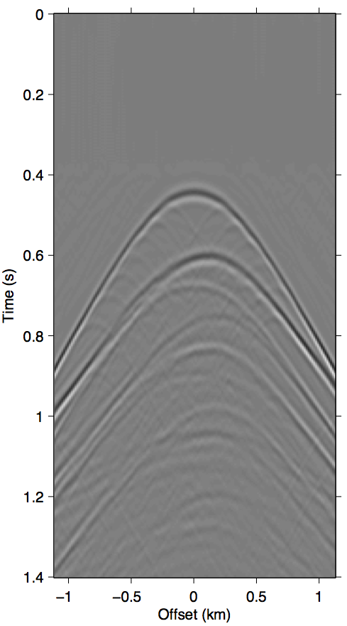
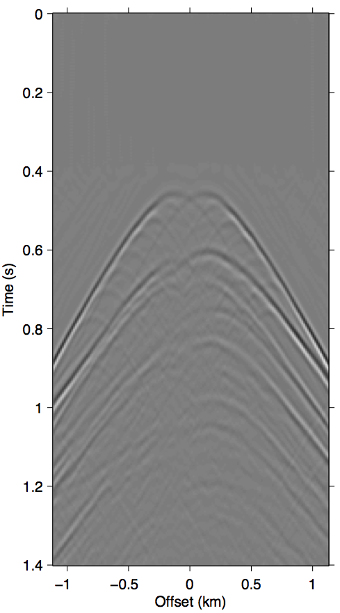
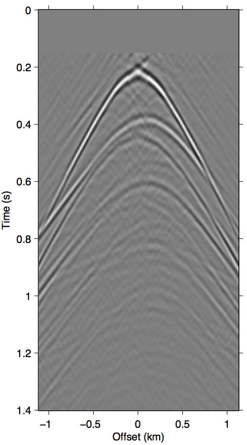
When the difference between \(\vec{p}\) and \(\vec{p'}\) is large, the incomplete coverage can become a significant source of error in the calculation of the surface multiples, especially at the near-offset locations (D. J. Verschuur, 2006). The most well-known example of this is missing near-offsets, as illustrated in Figure 2. The effects of these gaps on the multiple model are felt throughout the wavefield volume due to the surface integral that underlies the prediction process, which results in a non-stationary spatial convolution.

The approximation \(\vec{G} \approx \vec{P}\) that SRME doubles the impact of missing data during acquisition. Comparing Figure 1d with Figures 2b and 2c, it is clear that using \(\vec{P'}\) in place of \(\vec{G}\) greatly exasperates kinematic errors in the multiple prediction, resulting in completely unrecognizable wavefronts even when we have data available up to 100 m. Due to this effect, SRME usually requires some type of trace interpolation as a preprocessing step, since adaptive subtraction alone is not able to account for this degree of error.

However, on the flip side, the non-local effect of the prediction error ultimately enables us to probe the (actions of the) free surface inside the data gap based solely on measurements outside of it. Since EPSI inherently relies on wavefield inversion, there is enough degrees of freedom in the process to take advantage of this. Groenestijn and Verschuur (2009) proposes to explicitly reconstruct \(\vec{p''}\) from intermediate estimates of \(\vec{g}\), such that the accuracy of \(M\) improves as the algorithm converges. Adapting this approach to the REPSI formulation means extending the definition of \(\Mfreq\) with the unobserved traces as another variable in the forward modeling operator \[ \begin{equation} \Mfreq(\vector{G},\vector{Q},\vector{P''};\vector{P'}) := \vec{G}\vec{Q} + \vec{G}\vec{R}(\vec{P'} + \vec{P''}), \label{eq:normal_modeling} \end{equation} \] which leads to a more complicated version of problem \(\ref{eq:EPSIopt}\), with \(\vec{p''}\) as an additional unknown: \[ \begin{gather} \label{eq:EPSIopt_uP} \min_{\vector{g},\;\vector{q},\;\vector{p''}}\|\vector{g}\|_1 \quad\text{subject to}\quad f(\vec{g},\vec{q},\vec{p''};\vec{p'}) \le \sigma,\\ \nonumber f(\vec{g},\vec{q},\vec{p''};\vec{p'}) := \|\vector{p'} + \vec{p''} - M(\vector{g},\vector{q},\vector{p''};\vec{p'})\|_2. \end{gather} \]

A major issue with this method of independently updating \(\vec{g}\) and \(\vec{p''}\) in a cyclically alternating fashion is that we end up needing to include the intermediate and incorrect estimates of \(\vec{p''}\) into the observation term of the misfit functional. Otherwise, the parts of \(\vec{G}\) inside the unobserved locations will tend to converge very slowly, if at all, since its gradients would not be driven by the residuals that belong to the primaries, which only appears in \(\vec{p''}\) inside the gap.

This approach also ignores the fact that \(\vec{g}\) and \(\vec{p''}\) are tightly coupled in an obvious way. The strongest parts of these two wavefields (the primaries) overlap and relate to one another through convolution with the wavelet. The full relation is implicitly defined by \[ \begin{equation} \vec{P''} = \vec{K_c}\vec{P} = \vec{K_c}\big[\vec{GQ} + \vec{GRP'} + \vec{GRP''}\big] \label{eq:uP_recursive} \end{equation} \] where it is evident that \(\vec{P''}\) can be almost completely characterized by \(\vec{G}\). Therefore, we would expect that \(\partial\vec{p''}/\partial\vec{g}\) and \(\partial\vec{g}/\partial\vec{p''}\) should not be ignored when independently updating \(\vec{p''}\) and \(\vec{g}\). While \(\partial\vec{p''}/\partial\vec{g}\) is straightforward to compute, the expression for \(\partial\vec{g}/\partial\vec{p''}\) is, conversely, quite tricky and necessarily involves \(\vec{Q}^{-1}\) (deconvolution by the unknown wavelet function \(\vec{q}\)). Motivated by this observation, in this paper we seek to remove \(\vec{p''}\) as an inversion variable all-together, and instead account for its multiple contribution with terms that only involve \(\vec{g}\), \(\vec{q}\), and the known data \(\vec{p'}\).

Deterministic correction of surface multiple prediction by scattering terms

We start by attempting to eliminate \(\vec{p''}\) from the EPSI modeling function (expression \(\ref{eq:normal_modeling}\)) by recursively substituting it with the right-hand side of expression \(\ref{eq:uP_recursive}\). This results in a new modeling function that does not depend on \(\vec{p''}\), but at the cost of having infinitely many terms in a series expansion \[ \begin{align} \nonumber \widetilde{\Mfreq}(\vec{G},\vec{Q};\vec{P'}) &= \vec{K}\big[(\vec{GQ} + \vec{GRP'})\\ \label{eq:1stTerm} &\quad\;\;+\;\vec{GRK_c}(\vec{GQ} + \vec{GRP'})\\ \label{eq:2ndTerm} &\quad\;\;+\;\vec{GRK_c}\left(\vec{GRK_c}(\vec{GQ} + \vec{GRP'})\right)\\ \nonumber &\quad\;\;+\;\Order(\vec{G}^4)\big]\\ \label{eq:inftySeries} &:= \vec{K}\sum_{n=0}^{\infty}\left(\vec{GRK_c}\right)^n \left(\vec{GQ+GRP'}\right). \end{align} \] This expression is no longer linear in \(\vec{G}\). The \(n{=}1\) term (Equation \(\ref{eq:1stTerm}\)) is a second-order term since it is effectively a function of \(\vec{G}^2\), and similarly the \(n{=}2\) term (Equation \(\ref{eq:2ndTerm}\)) is a third-order term.

Since multiples that we observe in nature will decay in amplitude as a function of its order, we can assume from physical arguments that the spectral norm (i.e., largest singular value) of \(\vec{G}\) is \(\|\vec{G}\| < 1\), and therefore the infinite-term series expansion \(\ref{eq:inftySeries}\) converges to \[ \begin{equation} \vec{K}\vec{P} = \vec{K}\left(\vec{I - GRK_c}\right)^{-1} \left(\vec{GQ+GRP'}\right). \label{eq:autoconvSum} \end{equation} \] This expression states that we can recover the original EPSI forward model \(\vec{P} = \vec{GQ + GRP' + GRP''}\) if it is somehow possible to invert the data mask \(\vec{K}\) by some hypothetical exact data interpolation, which validates our recursive substitution derivation above.

Although Equation \(\ref{eq:autoconvSum}\) is not practically useful, it admits an useful interpretation of our approach: that of a Born series solution to a Lippmann-Schwinger relation between the total wavefield \(\vec{P}\) and an “incident wavefield” composed of the erroneous EPSI prediction \(\left(\vec{GQ+GRP'}\right)\) from incomplete data. The perturbation in this case is the missing contribution coming from within the acquisition gap. This view makes it clear that each term in expression \(\ref{eq:inftySeries}\) is a term in the Born series expansion due to the free-surface reflector within the confines of the acquisition gap (as bound by the stencil \(\vec{K_c}\)). One direct consequence of this interpretation is that we can expect all orders of surface multiples in every term of expression \(\ref{eq:inftySeries}\), because the incident wavefield is not only composed of the primaries \(\vec{GQ}\) but also parts of all subsequent orders of surface multiples, as produced by the term \(\vec{GRP'}\).

This scattering-based interpretation is perhaps most commonly seen in literature on the inverse scattering series (ISS) approach to multiple removal (Weglein et al., 1997, 2003). However, unlike typical applications of ISS methodology where it is used on subsurface reflectors for internal multiple removal, in this paper we know exactly that the scattering boundary is at the free surface, and have only reflection effect from this scatterer. Perhaps more significantly, we use the derived multiples as part of the modeling function in the context of a full data-fitting inversion problem for the primary estimation, instead of an adaptive subtraction scheme.

As with all series expansion expressions, it is important to investigate how the approximation error behaves as a function of the number of terms used. Since computing these terms involve partial wavefield convolutions that have significant computation costs (although not as much as the full wavefield convolution, as we will discuss later in the paper), it is practically desirable to limit the number of terms as much as possible. We now claim what is perhaps the main insight of this paper: that a very small number of these terms, even just two or three, can be enough to account for most of the missing multiple contributions.

Effects of term truncation on accuracy

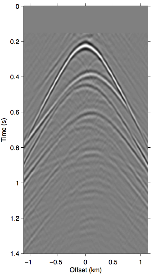
As discussed in the previous section, the whole series up to the \(n\)-th term of expression \(\ref{eq:inftySeries}\) accounts for all of the missing \(n\)-th order multiples coming from the part of the free surface confined within the acquisition gap. It also includes some part of all multiples of \(n{+}1\)-th order and above, although for near-offset gaps these contributions may be small. Figure 3 shows this with shot-gather representations of the different terms in expression \(\ref{eq:inftySeries}\) for the synthetic dataset shown in Figure 2a. We can see that the majority of these terms is composed of the \(n\)-th order surface multiple by comparing the wavefront shapes and traveltimes of panels 3b and 3c to the true primaries shown in Figure 1c. The arrows in panel 3b shows two apexes of the missing contribution of the second-order surface multiple, which we can see faintly in the \(n{=}1\) term (Equation \(\ref{eq:1stTerm}\)) and very prominently the \(n{=}2\) term (Equation \(\ref{eq:2ndTerm}\)). The sum of these two terms, shown in panel 3d, perfectly accounts for the total missing contribution to the wavefront without relying on any data inside the gap.

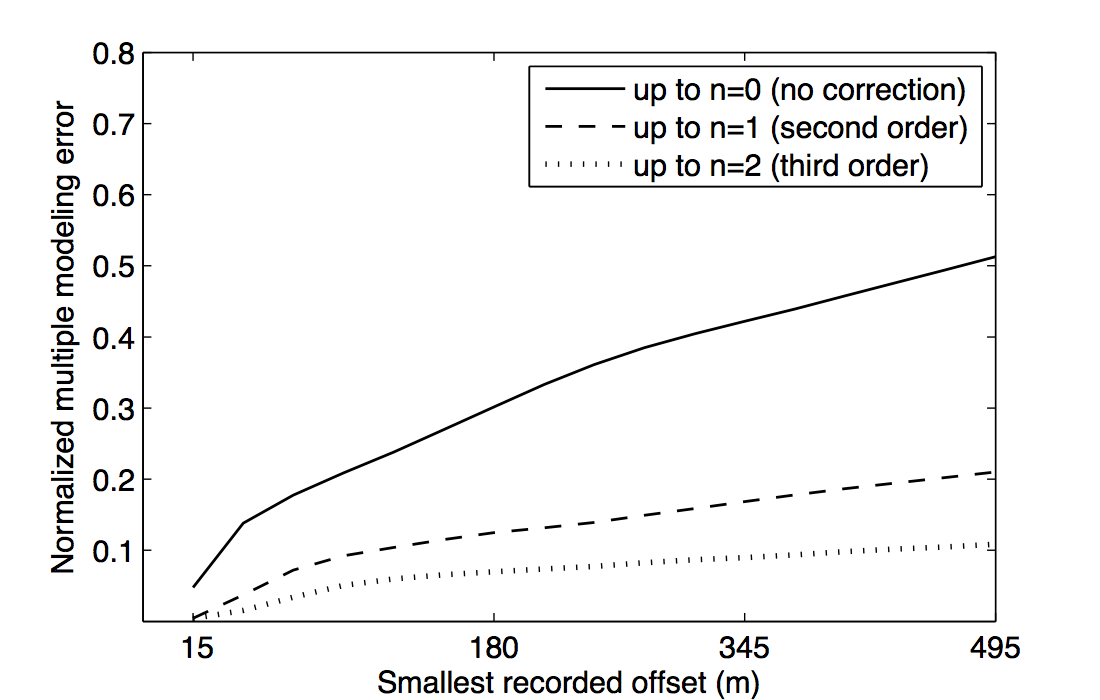
Figure 3 also visually demonstrates that the sum of just the first three terms of the series expansion \(\ref{eq:inftySeries}\) is enough to model most of the significant multiple contributions from the missing data \(\vec{p''}\). Panel 3d, which shows the sum of the \(n{=}1\) and \(n{=}2\) terms, explains all the missing contributions from \(\vec{p''}\) (panel 3a) up to the second-order surface multiple, and also contains some kinematic imprints of all higher order ones. Together, these two terms were able to bring the normalized prediction error (defined by \(\|\vec{p}_m - \widetilde{M}(\vec{g},\vec{q};\vec{p'})\| / \| \vec{p}_m \|\), where \(\vec{p}_m\) is the true surface multiple) down from \(\approx\)22% down to \(\approx\)3%. Figure 4 summarizes the effectiveness of these first two terms as a function of the nearest available offset.

From the general trend of the curves in Figure 4 we can see that, for a range of typical near-offset gap sizes, just including the \(n{=}1\) term can reduce the normalized multiple modeling error of \(\widetilde{M}\) by more than one half (corresponding to a 6 dB improvement), and a further halving of the error is achieved by including up to the \(n{=}2\) term. The model used here the same ones as used by Groenestijn and Verschuur (2009), with a gently-varying water column depth around 200 m throughout the model, and a water-bottom reflectivity coefficient of \(\approx\)0.41 (seafloor p-wave velocity 2.0 km/s, density 1.8 g/cm³).

Algorithmic considerations

With the new augmented forward-modeling operator \(\widetilde{M}(\vec{G},\vec{Q};\vec{P'})\) as defined in Equation \(\ref{eq:inftySeries}\) using data-matrix notation, we solve a new optimization problem by using it in place of the uncorrected modeling operator in the original REPSI problem (c.f. Equation \(\ref{eq:EPSIopt_uP}\)): \[ \begin{gather} \label{eq:EPSIopt_autoconv} \min_{\vector{g},\;\vector{q}}\|\vector{g}\|_1 \quad\text{subject to}\quad f(\vec{g},\vec{q};\vec{p'}) \le \sigma,\\ \nonumber f(\vec{g},\vec{q};\vec{p'}) := \|\vector{p'} - \widetilde{M}(\vector{g},\vector{q};\vec{p'})\|_2. \end{gather} \] The main challenge that we will address in this section is that, compared to the original REPSI problem with fully-sampled data, this new one loses the linear relationship of the modeling function with \(\vec{g}\). In Lin and Herrmann (2013), we relied on this bilinear property of \(M(\vec{g},\vec{q};\vec{p'})\) in terms of \(\vec{g}\) and \(\vec{q}\) to solve problem \(\eqref{eq:EPSIopt}\) using an alternating coordinate-descent method. Below we first briefly recount how the original REPSI problem is solved, followed by the proposal of two possible ways to modify our solution strategy to account for the additional nonlinearity due to the existence of higher-order terms in \(\widetilde{M}(\vec{G},\vec{Q};\vec{P'})\).

The existing approach to solving the original REPSI problem \(\eqref{eq:EPSIopt}\) is an alternating update of \(\vec{g}\) and \(\vec{q}\). Each new iteration of \(\vec{g}\) is formed by a \(\ell_1\)-norm constrained problem (called a Lasso problem, Tibshirani, 1996) to give a sparse wavefront, which has a broadband, impulsive appearance in time. We then use it to estimate the wavelet \(\vec{q}\) by matching the impulsive wavefronts against the data. The number of sparse wavefronts allowed into \(\vec{g}\) is kept small at the early iterations to capture only the most significant primary events, quickly giving us the best estimate for the wavelet \(\vec{q}\). Later iterations will then gradually increase the number of events allowed to better fit the remaining data residual.

This relaxation of sparsity constraint happens in a theoretically rigorous way for REPSI. The sparsity of \(\vec{g}\) is directly influenced by the \(\ell_1\)-norm constraint value of the Lasso problems. The initial \(\ell_1\)-norm constraints start at a small value that is designed to be an underestimate of the true minimum. It is then is gradually increased throughout the iterations in a way such that it does not exceed the \(\ell_1\)-norm of the true solution, yet approaches it quickly. This scheme is enabled by the convex properties of the Pareto trade-off curve for Lasso problems (E. van den Berg and Friedlander, 2008; Hennenfent et al., 2008; Daubechies et al., 2008).

We now roughly outline the main algorithm as described in Lin and Herrmann (2013), using the notation of this paper and omitting some initialization details. We first set our solution candidates \(\evec{p}_0\) and \(\evec{q}_0\) to zero vectors, and the inversion residue (prediction error) \(\vec{e}\) to \(\vec{p}\). Then we iterate over the following steps with iteration counter \(k\).

1. Select a new \(\ell_1\) norm constraint \(\tau_k > \tau_{k{-}1}\), which is evaluated through a closed-form expression from the current residue \(\vec{e}_k\), the target misfit \(\sigma\), and the \(\ell_1\)-norm of the current solution \(\vec{g}_k\).

2. Obtain \(\vec{g}_{k+1}\) by solving through a spectral projected gradient method (E. van den Berg and Friedlander, 2008; Birgin et al., 2000), using the previous solution \(\vec{g}_k\) as the initial guess \[ \begin{equation} \min_\vec{g} \|\vector{p} - M(\vector{g},\vector{q}_k;\vector{p})\|_2\;\text{subject to}\;\|\vec{g}\|_1<\tau_k. \label{lasso_EPSIsubproblem} \end{equation} \]

3. Do an exact line-search scaling on \(\vec{g}_{k+1}\) using the multiple term in \(M(\vector{g},\vector{q}_k;\vector{p})\) on \(\vec{p}\) to minimize the effect of the \(\ell_1\) constrain on the amplitude of \(\vec{g}_{k+1}\).

4. Obtain \(\vec{q}_{k+1}\) by solving a matched-filtering problem \[ \begin{equation*} \min_\vec{q} \|\vector{p} - M(\vector{g}_{k+1},\vector{q};\vector{p})\|_2\ \end{equation*} \]

5. Form a new residue \(\vec{e}_{k+1} = \vec{p} - M(\vector{g}_{k+1},\vector{q}_{k+1};\vector{p})\) and check for convergence conditions.

6. (If explicitly reconstructing data as in Problem \(\ref{eq:EPSIopt_uP}\)) Solve for the missing part of the data \(\vec{p''}_{k{+}1}\), using the previous solution \(\vec{p''}_k\) as the initial guess \[ \begin{equation*} \min_\vec{p''} \|\vector{p'} + \vector{p''} - M(\vector{g},\vector{q}_k;\vector{p'} + \vector{p''})\|_2 \end{equation*} \] and form new data by \(\vec{p} = \vec{p'} + \vec{p''}_{k{+}1}\).

For steps 1 and 2 we depend on the notion of a smooth, monotonic Pareto curve (sometimes known as the L-curve) for problem \(\ref{eq:EPSIopt}\) to give us sensible \(\ell_1\)-norm constraint parameters \(\tau_k\). The smooth and monotonic property is generally no longer valid when the forward system is nonlinear in \(\vec{g}\), so below we will discuss two possible approaches to work around this issue, and propose how it can be applied to the above strategy to derive suitable methods for solving \(\ref{eq:EPSIopt_autoconv}\).

Modified Gauss-Newton approach

Several existing works on regularized inversion of auto-convolution functions rely on either the Gauss-Newton method or more generally the Levenberg-Marquardt method (Fleischer et al., 1999; Fleischer and Hofmann, 1996). In the same vein, we introduce an approach inspired by Li et al. (2012), which gives heuristically sparse solutions to the new nonlinear REPSI problem \(\eqref{eq:EPSIopt_autoconv}\) using a modified Gauss-Newton method.

The crux of this method is to always ensure that the Green’s function updates \(\Delta\vec{g}\) are as sparse as possible for our a given amount of decrease in the objective. This is achieved most effectively by taking as updates the solution to a Lasso problem formed around the Jacobian \(\vec{J}_k\) of \(\widetilde{M}\) evaluated at \((\vec{g}_k,\vec{q}_k)\): \[ \begin{equation} \Delta\vec{g}_{k+1} = \mathop{\mathrm{argmin}}_{\vec{g}} \| \vec{e}_k - \vec{J}_k\vector{g}\|_2 \quad\text{s.t.}\quad\|\vector{g}\|_1 \le \tau_k, \label{lasso_mGN} \end{equation} \] where \(\vec{e}_k\) is the current nonlinear residue \(\vec{p} - \widetilde{M}(\vec{g}_k,\vec{q}_k)\). The \(\ell_1\)-norm constraint \(\tau_k\) in this case is again obtained deterministically by the optimization parameters of problem \(\ref{lasso_mGN}\), using the same expressions used in step 1. However, since we are explicitly solving for updates \(\Delta\vec{g}\) instead of \(\vec{g}\) itself, the previous solution \(\vec{g}_k\) (and hence its \(\ell_1\)-norm) for this linearized problem is always zero. Each update formed this way will thus tend to have a much smaller \(\ell_1\)-norm constraint \(\tau_k\) compared to the final \(\ell_1\)-norm of the true solution, but the sum of all the updates may have a final norm that exceeds it. The assumption here is that our series of sparse updates will actually sum into a sparse final solution, which will depend on the Jacobians evolving slow enough over the iterations, so that all updates \(\Delta\vector{g}\) kinematically all consists of very similar wavefront sets. In practice, we find that this assumption is rarely a problem if the acquisition gaps are not too large, and that we indeed usually end up with sparse solutions for \(\vector{g}\).

The action of the Jacobian \(\vec{J}_{k}\) is straightforward to obtain, but actually computing it will pose a challenge. When we explicitly write it out using the data-matrix notation, it becomes evident that the computational effort required escalates very quickly with the order of the series expansion: \[ \begin{equation} \begin{aligned} \vec{J}_{k\omega} \vec{G} = \vec{K}\big[(&\vec{G}\vec{Q}_k + \vec{GRP'}) \\ +\;&\vec{G}_k\vec{R}\vec{K_c}(\vec{G}\vec{Q}_k + \vec{G}\vec{RP'}) \\ +\;&\vec{G}\vec{R}\vec{K_c}(\vec{G}_k\vec{Q}_k + \vec{G}_k\vec{RP'}) \\ +\;&\vec{G}_k\vec{R}\vec{K_c}\left(\vec{G}_k\vec{R}\vec{K_c}(\vec{G}\vec{Q}_k + \vec{G}\vec{RP'})\right) \\ +\;&\vec{G}\vec{R}\vec{K_c}\left(\vec{G}_k\vec{R}\vec{K_c}(\vec{G}_k\vec{Q}_k + \vec{G}_k\vec{RP'})\right) \\ +\;&\vec{G}_k\vec{R}\vec{K_c}\left(\vec{G}\vec{R}\vec{K_c}(\vec{G}_k\vec{Q}_k + \vec{G}_k\vec{RP'})\right) \\ +\;&...\big]. \end{aligned} \label{autoconvM_jacobian} \end{equation} \] The above expression is only written up to the \(n{=}2\) nonlinear term (expression \(\ref{eq:2ndTerm}\)) of \(\widetilde{M}\). Comparing all the terms here to the original nonlinear expression \(\ref{eq:inftySeries}\), we can see that due to partial derivatives, each of the \(\Order(\vec{G}^n)\) terms expand into \(n\) linearized terms in the Jacobian. In aggregate, this effectively introduces a quadratic complexity in the number of nonlinear terms when computing the action. Although some reuse is possible in the calculation of these terms, this approach may nonetheless present a prohibitive amount of computation overhead compared to the original problem. In the next subsection we will discuss an alternative scheme that forgoes using the Jacobian and will instead linearize the problem in some other way.

To summarize the modified Gauss-Newton approach to solving problem \(\ref{eq:EPSIopt_autoconv}\), we essentially modify steps 2 and 3 of the original algorithm above. In step 2 of each iteration we explicitly compute the updates \(\vec{g}_{k+1} = \vec{g}_{k} + \Delta\vec{g}_{k+1}\) with \(\Delta\vec{g}_{k{+}1}\) given by solving problem \(\ref{lasso_mGN}\). In step 3 we then perform the exact line-search on the update \(\Delta\vec{g}_{k+1}\) itself against the current residual, much like in the original algorithm, this mitigates the amplitude loss from the \(\ell_1\)-norm regularization while keeping its sparsifying effect.

Relinearization by substitution

As shown in expression \(\ref{autoconvM_jacobian}\), having to compute the action of the Jacobian of the operator \(\widetilde{M}\) may be unacceptably costly, considering that each wavefield multiplication in these expressions is computationally equivalent to one full SRME multiple prediction step. Since our non-linearity only comes from essentially having quadratic and higher powers of \(\vec{G}\), a possible alternative to avoid dealing with the Jacobian is to simply substitute the previous iteration \(\vec{g}_{k}\) as a constant in the \(\left(\vec{GRK_c}\right)^n\) part of Equation \(\ref{eq:inftySeries}\). This returns us to the paradigm of inverting a linear operator in \(\vec{G}\) at step 2: \[ \begin{equation} \begin{aligned} \widetilde{M}_{k\omega}(\vec{G}) = \vec{K}\big[(&\vec{G}\vec{Q}_k + \vec{GRP'}) \\ +\;&\vec{G}_k\vec{R}\vec{K_c}(\vec{G}\vec{Q}_k + \vec{GRP'}) \\ +\;&\vec{G}_k\vec{R}\vec{K_c}\left(\vec{G}_k\vec{R}\vec{K_c}(\vec{G}\vec{Q}_k + \vec{GRP'})\right) \\ +\;&...\big]. \end{aligned} \label{autoconvM_relin} \end{equation} \]

Similar to Gauss-Netwon, the approach also relinarizes the problem at step 2, except that we do not have to find each update explicitly. Instead, we simply replicate step 2 of the original REPSI algorithm (solving the Lasso problem in Equation \(\ref{lasso_EPSIsubproblem}\) starting from the previous solution \(\vec{g}_{k}\)) using the approximate but linear modeling operator of expression \(\ref{autoconvM_relin}\). In effect, we now solve the following in step 2: \[ \begin{equation} \min_\vec{g} \|\vector{p} - \widetilde{M}_{k}(\vec{g})\|_2\;\text{subject to}\;\|\vec{g}\|_1<\tau_k. \label{lasso_relinearization} \end{equation} \]

Theoretically speaking, we have to give up some nice properties of Gauss-Newton with this method, such as possible quadratic convergence and guarantees of reaching a stationary point. But in practice we find this method, which we call “relinearization” for the purpose of this paper, to converge similarly to the Gauss-Newton approach while also having much smaller per-iteration compute costs. In fact, the computational overhead here is marginal compared to the original algorithm, as we explain in the Discussions section. However, to achieve this result we find that it is necessary to manually precondition the first few gradients, where we have zero contribution coming from the missing primary part of \(\vec{p''}\).

Improving convergence by gradient trace weighting

If we explicitly write out a (negative) gradient step of the Lasso problem in step 2 (where the residue is at \(\vec{e}_k\)) using the approximate operator in expression \(\ref{autoconvM_relin}\) up to the \(n{=}1\) term, we obtain, assuming \(\vec{R} = -\vec{I}\) and using \(H\) for Hermitian adjoint, \[ \begin{equation*} (\vec{KE}_k)\vec{Q}_k^H - (\vec{KE}_k)\vec{P'}^H - \vec{K_c G}_k^H(\vec{KE}_k)\vec{Q}_k^H + \vec{K_c G}_k^H(\vec{KE}_k)\vec{P'}^H. \end{equation*} \] Recall that \(\vec{E}_k\) is the data-matrix representation of the current residue error \(\vec{e}_k\). From this we can see that \(\vec{g}\) is not being updated equally inside the acquisition mask compared to the outside of it. In fact, the first term is actually zero inside the acquisition mask (i.e., \(\vec{K_c}\vec{K} = 0\) so \(\vec{K_c}(\vec{KE}_k)\vec{Q}_k^H = \vec{0}\)), due to the residue being zero inside the mask, and the fact that the source wavelet applies a purely time domain convolution which does not spatially “spread” the wavefield. Since this term contains all the contribution from primary wavefields, which tends to be the strongest part of the wavefield, there is immediately a large loss of amplitude for the updates inside the mask. The job of filling this void then naturally falls to the subsequent terms, which all involve some sort of wavefield convolution and can potentially generate events inside the mask. However, in the first few gradients where \(\vec{G}_k\) is small in amplitude (due to the \(\ell_1\)-norm constraints), the third term and above are also unhelpfully close to zero. This creates a convergence “lag” where traces of \(\vec{g}\) outside of the mask must already be well reconstructed in order for the inside of the mask to begin updating, which is problematic because the outside traces are susceptible to overfit on multiples that should ultimately be explained by contributions coming from the inside of the mask.

We can mitigate the inherent imbalance on the early gradients through a simple weighting to all traces inside the acquisition gap. This can be seen as applying a diagonal right preconditioner to the linearized modeling operator. For the Gauss-Newton approach, this kind of scaling is automatically handled by the implicit Hessian, but for the relinearization method we must form and apply this preconditioner manually. An averaged, trace-independent version can be obtained by finding an exact line-search for a scaling \(\alpha\) of \(\vec{K_c}\vec{g}_{k+1}\) which maximally reduces the residual left over from the contributions of \(\vec{K}\vec{g}_{k+1}\) under the action of the next forward operator \(\widetilde{M}_{k+1}\) (not that it is linearized around the newly obtained \(\vec{g}_{k+1}\)). In other words, we seek the scalar \(\alpha\), which solves the following problem \[ \begin{equation*} \min_{\alpha} \|\big(\vector{p'} - \vec{K}\widetilde{M}_{k+1}(\vec{K}\vec{g}_{k+1})\big) - \alpha\vec{K}\widetilde{M}_{k+1}(\vec{K_c}\vec{g}_{k+1})\|_2^2. \end{equation*} \] The computation of this scaling can be effectively free in the process of computing the residual of iteration \(k{+}1\), by producing the new predicted wavefield due to the two parts of \(\vec{g}_{k+1}\) separately: \[ \begin{align} \nonumber \vec{e}_\text{outside} &= \vec{p'} - \vec{K}\widetilde{M}_{k+1}(\vec{K}\vec{g}_{k+1})\\ \nonumber \evec{p}_\text{inside} &= \vec{K}\widetilde{M}_{k+1}(\vec{K_c}\vec{g}_{k+1})\\ \label{relin_precond_scaling} \alpha_{k+1} &= \evec{p}_\text{inside}^T\vec{e}_\text{outside}/ \|\evec{p}_\text{inside}\|_2^2. \end{align} \] Note that all the computational cost for this scaling is in the last line, which only involves the vector inner products between \(\evec{p}_\text{inside}\) and \(\vec{e}_\text{outside}\), as well as \(\ell_2\) norms. All the terms needed to form these two wavefields are already computed once we have the final residue for this iteration. As an aside, this scaling should be calculated after the line-search over all of \(\vec{g}\) described in step 3, to minimize the impact of the accuracy of the current wavelet estimate (simply ignoring the primary \(\vec{GQ}\) term when forming \(\evec{p}_\text{inside}\) and \(\vec{e}_\text{outside}\) will have a similar effect).

After obtaining \(\alpha\), we use it as a right-preconditioner \(\alpha\vec{K_c}\) in step 2 of the next iteration, where we now solve \[ \begin{equation} \min_{\evec{g}} \|\vector{p} - \widetilde{M}_{k}(\alpha\vec{K_c}\evec{g})\|_2\;\text{subject to}\;\|\evec{g}\|_1<\tau_k. \label{lasso_relinearization_precond} \end{equation} \] This will effectively scale all gradient traces inside the stencil by \(\alpha\). After the inversion is complete, we obtain the new estimate of the Green’s function by \(\vec{g}_{k{+}1} = \alpha\vec{K_c}\evec{g}\), which removes the imprint of the right preconditioner. As the iteration count increases and \(\vec{g}\) becomes more accurate, we should see \(\alpha\) trend towards 1.

Figure 5 demonstrates the effectiveness of this method. Panel 5a shows the first gradient update for \(\vec{g}\) (assuming we use the true wavelet \(\vec{q}\)) we would have obtained from a full-sampled data (shown in Figure 1a). Panel 5b shows the same gradient step that we would obtain using data with missing near-offsets (Figure 2a). We can see that this update contains mostly correct kinematic information about the wavefield, but is much weaker in amplitude for traces inside the near-offset gap. After applying the preconditioner \(\alpha\vec{K_c}\), with \(\alpha\) computed using the inaccurate gradient in Panel 5b as the approximate solution, we see in Panel 5c that this amplitude imbalance is effectively mitigated.

To summarize, in the “relinearization” approach we essentially replace the steps 2 and 3 of the original algorithm with the following modified steps:

2. Solve the modified Lasso problem (Equation \(\ref{lasso_relinearization_precond}\)) instead of the original one (Equation \(\ref{lasso_EPSIsubproblem}\)). This replaces the wavefield modeling function with the approximately linearized version of \(\widetilde{M}\), defined in expression \(\ref{autoconvM_relin}\), and adds a right preconditioner \(\alpha_{k}\vec{K_c}\). Once solution is obtained, apply \(\alpha_{k}\vec{K_c}\) to invert the preconditioner and get \(\vec{g}_{k{+}1}\).

3. Compute the scaling for all of \(\vec{g}_{k{+}1}\) as in the original. After applying the scaling, compute the next preconditioner scaling \(\alpha_{k{+}1}\) using expression \(\ref{relin_precond_scaling}\).

Numerical examples

In this section we demonstrate the efficacy of our proposed methods, focusing on the missing near-offset problem. We compare the results given by both the Gauss-Newton and the relinearization approach, using up to the \(n=2\) term (expression \(\ref{eq:2ndTerm}\)) in the augmented nonlinear modeling operator \(\widetilde{M}(\vector{g},\vector{q};\vec{p'})\). We also compare our results to the explicit data reconstruction approach (problem \(\ref{eq:EPSIopt_uP}\)) based on the method suggested by Groenestijn and Verschuur (2009), as well as a parabolic Radon-domain interpolation done as a preprocessing step. We first show results using the synthetic data shown in 1a, then move on to a field data example from the North Sea. Although we only show 2D acquisition examples, note that our method makes no assumptions on the coordinate system used for the data matrices, so it is trivially extendable to a 3D survey geometry.

Synthetic data example

In this section we focus on how effectively the proposed methods in this paper handle different sizes of near-offset gaps, and how it fares compared to explicitly inverting for the missing data \(\vec{p''}\). We use the same 5 km fixed-spread synthetic data used in all the figures so far in the paper, a shot gather of which is shown in Figure 1a. For reference, the corresponding true primary model is shown in Figure 1c. This model appears in almost all existing EPSI literature today and serves as an effective benchmark.

Figure 6 shows a comparison of methods for a 45 m near-offset gap (in both positive and negative offsets). This is an extremely mild offset gap and typically poses no major problems for SRME workflows. In this case, the data reconstruction (Panel 6b), the Gauss-Newton (Panels 6c and 6d), and the relinearization strategies (Panel 6e) all performed very similarly and gave good results without needing to interpolate the near-offsets in preprocessing. All the results plotted here is the direct primary estimation (the final \(\vec{g}\) from the inversion convolved with the final \(\vec{q}\) from the same inversion), as the effects of reconstruction inside the offset gap is clearer this way. In practical applications, usually a multiple model would be formed with the solution \(\vec{g}\) instead, so it can be subtracted from the data under perhaps more scrutiny.

Comparing the Gauss-Newton results allows us to examine the effects of term truncation in the nonlinear modeling operator \(\widetilde{M}\). Panel 6c shows the Gauss-Newton solution using up to the \(n{=}1\) term (second-order in \(\vec{g}\)) in \(\widetilde{M}\). As discussed in the theoretical section, this term alone cannot fully account for the second-order surface multiples, and thus some part of the first order multiple is put into \(\vec{g}\) by the algorithm to make up some of the difference. This is especially apparent inside the offset gap, where \(\vec{g}\) is less constrained by the observed data.

Panel 6d shows the solution we can obtain by just using one more term in \(\widetilde{M}\), up to the \(n{=}2\) term which is third-order in \(\vec{g}\). We see that the imprint from the first-order multiple is much less severe in this result. This result, notably, is already very close to the solution from fully sampled data as shown in Figure 1c, even though only two additional terms from the series expansion is used. The results of the relinearization method (also using up to the \(n{=}2\) term) shown in Panel 6e is almost identical to the Gauss-Newton solution, despite being much faster to compute. In fact it is arguably cleaner, perhaps due to less overfit of the remaining multiple prediction errors from the lack of higher order terms.

Figure 7 shows the opposite end of the near-offset gap severity scale with a 225 m offset gap. As we can see in panel 7a, the majority of the near-offset wavefront curvature information is missing, which poses a serious challenge for standard workflow tools to accurately reconstruct near-offset traces. In this case the explicit data reconstruction (Figure 7b) fails to remove some of the later surface multiples, such as those after 0.6 s. The augmented nonlinear modeling operator approach introduced in this paper all arguably fared better in comparison. The Gauss-Newton approach up to the second-order term (Figure 7c) is better at recovering the wavefronts inside offset gap, even building up some of the diffraction events, but also similarly fails to remove some of the later surface multiples. The multiple removal is improved greatly by including up to the third-order term (Figure 7d), although some still remain, again possibly due to overfit. The relinearization method remains the overall winner in this case (Panel 7e), producing the cleanest primary estimation that is nearly identical to the reference primary outside of the near-offset gap, while also computing it much faster than the Gauss-Newton method.

Field data example

We now demonstrate the effectiveness of our proposed methods using a North Sea shallow-water marine 2D seismic line with a 100 m near-offset gap. Pre-processing has been applied to convert the collected dual-sensor data to an upgoing pressure wavefield using the method described in Cambois et al. (2009). Data regularization and interpolation were carried out as part of the preprocessing, so in this example we will compare our method with the existing parabolic Radon interpolated near-offsets. A 3D-to-2D correction factor \(\sqrt{t}\) has also been applied after data regularization.

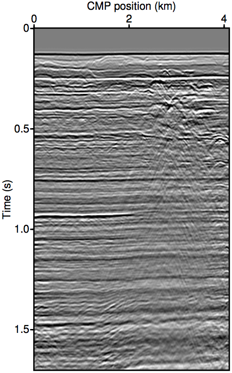
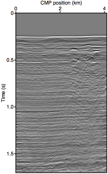
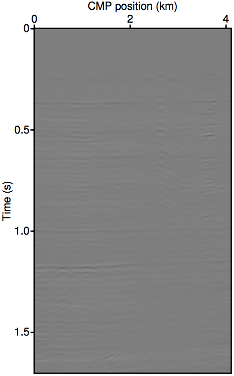
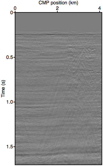
Figure 8 show the moveout-corrected stacks of the field data experiments. Panel 8a shows the data itself. All near-offsets are excluded from the stack to keep comparisons consistent. Panel 8b shows the results obtain from using the original REPSI on the regularized data where the near-offset is pre-interpolation using parabolic Radon. Panel 8c show results obtained by inverting the third order (keeping up to \(n{=}2\) terms) nonlinear operator \(\widetilde{M}(\vec{g},\vec{q};\vec{p'})\) using the relinearization method, while panel 8d shows the same using the Gauss-Newton method.

Our methods are successful at improving on the results obtained by using unmodified EPSI on pre-interpolation data. In shallow water data most pre-interpolation methods are known to be inaccurate, often under-estimating near-offset amplitudes and incorrectly assessing wavefront curvature at the apex. Comparing panel 8b with panels 8c and 8d shows that our methods exhibit a much improved ability to remove large water-bottom multiples that is evident at 0.25 s, 0.55s, and 0.8 s of the stack. This is especially evident by looking at the multiples removed from the pre-interpolation result (panel 8e) and comparing it to the multiples removed using the relinearization result (panel 8f). By discarding the pre-interpolated near-offset and using the augmented modeling operator \(\widetilde{M}\) to account for its effects, we are able to get a much better defined multiple model with more accurate amplitude. Pre-interpolation also led to some ringing kinematic artifacts in the multiple model near the large diffraction events at 3 km and 1.0 s, which is not present in our methods.

Panel 8g shows a difference plot between inverting the second order (keeping up to \(n{=}2\) terms) and the third order forward operator using relinearization. We see that the impact of using the additional term is already very small, and mainly consists of the imprint of second-order surface multiples. The comparison between relinearization and Gauss-Newton is more interesting (panel 8h). It is not very clear from the difference plot which method produced a better multiple model, although when carefully examining the primary stacks we see that the amplitude of the first water-bottom multiple (at 0.25 s) is slightly over-estimated for Gauss-Newton. This is possibly due to the over-fitting issues discussed earlier in the synthetic example section. Nevertheless, the relinearization method once again provided a very good result at a fraction of the compute time required for Gauss-Newton.

Discussion

The synthetic results shown in the previous section demonstrated that our proposed scattering-based correction to the multiple modeling with incomplete data can outperform the existing explicit data reconstruction approach used in literature, especially when larges gaps are encountered in the near-offset. As far as we are aware, our proposed method is also the first practical formulation where a scattering series is rigorously used in a variational problem for primary estimation, with all its numerical approximations explicitly stated and explored. The real data example also demonstrates a significant improvement over using parabolic Radon interpolation for the near-offset. These improvements are tangible regardless of the algorithmic approach used to invert the augmented and non-linear modeling operator.

Perhaps more interestingly, we find that the Gauss-Newton method did not converge appreciably faster than the conceptually simpler and computationally cheaper relinearization method, despite its more solid theoretical convergence guarantees. This might be because the number of total gradient updates typically involved in REPSI is already fairly small (typically around 50), since the projected gradient method that we employ to solve the Lasso problems forms an implicit Hessian of the problem by using spectral step lengths (Birgin et al., 2000). The Gauss-Newton Hession might not have ben able to improve much more on this scaling information. On the other hand, we find to our surprise that the relinearization strategy often produced better results. One possible explanation is that in some of the later iterations, the Gauss-Newton method is more prone to over-fitting \(\vec{g}\), particularly inside the trace mask where it is less sensitive to data misfit, to account for some of the inherent modeling error due to term truncation.

Although we have only shown near-offset acquisition gap effects in this paper, the derivations in this paper is valid for missing data located anywhere on the acquisition geometry. We impose no special structure on our diagonal masking operator \(\vec{K}\), so in theory the missing traces can be anywhere. Near-offset traces are well-understood to be responsible for the majority of the constructively interfering part of the multiple contribution gather, so we conveniently use it as a worst-case scenario where the presence of \(\vec{K}\) can introduce the largest errors.

In theory, our scattering-based method to account for missing data works only when we can trace ray paths that reaches the inside of the masked location from the observed data positions, using the estimated Green’s function. This would imply that missing traces near the edge of the acquisition grid would be less effectively mitigated, which we do observe in practice. However, we find that the resulting edge effects tend to be overshadowed in magnitude by what would typically be produced in imaging algorithms.

Another important exception to the generality of our method is that the methods in this paper cannot deal with regular undersampling, even if it strictly counts as missing data in our framework. This is mainly because the mechanisms employed here also depends on wavefield interferometry, which is fundamentally erroneous when strong, coherent spatial aliasing is present in the data.

Finally, we note that one additional advantage of our approach over explicit data reconstruction is the possibility of exploiting any existing regularization schemes for \(\vec{g}\), such as the curvelet-based estimation shown in Lin and Herrmann (2013), although a thorough investigation is outside the scope of this paper. This has the potential to improve the accuracy of the recovery inside the gap using constraints such as wavefront continuity and lateral smoothness. While it is also possible to regularize explicitly reconstructed data, it is much easier in our approach to take advantages of regularizations that are already in place.

Computation costs

In each of the scattering terms \(\vec{GRK_c}\) in expression \(\ref{eq:inftySeries}\), the wavefield convolution is done after stencilling out the traces that lie inside unobserved locations. Therefore the computation cost of applying each of the higher-order terms will depend on the ratio of unobserved to observed locations, and can be much smaller than the convolution cost for the whole wavefield if we are only interested in near-offsets. Since we only have to apply a single \(\vec{GRK_c}\) to the current term to obtain the subsequent subsequent term, the marginal cost of using higher-order terms is small, and the aggregate cost of computing expression \(\ref{eq:inftySeries}\) will only be a fractional overhead to the uncorrected modeling operator.

The story is different when applying the adjoint of the relinearized operator (expression \(\ref{autoconvM_relin}\)) to form the gradient for \(\vec{g}\) in the relinearization step. In this case each of the scattering terms add a \(\vec{K_cR}^H\vec{G}^H\) to the previous-order term. Although we still involve the stencil \(\vec{K_c}\) before computing the next term, there is a special case when computing the \(n{=}1\) term, where we do not have a stencil between \(\vec{G}^H\) and the residual wavefield, and instead need to compute one full wavefield convolution over the whole grid. The cost of the (linearized) adjoint is thus two times the cost compared to the uncorrected modeling operator, plus the same fractional overhead for higher order terms as in the forward.

However, note that the method in this paper avoids the cost of updating and store the unknown data \(\vec{p''}\) as described in step 6 of the original algorithm. The gradients for \(\vec{p''}\) also require a full wavefield convolution, so the overall cost of updating the unknown wavefield is actually absorbed into the cost of updating \(\vec{g}\). In fact, if we only use the \(n{=}1\) term, then the overall computational cost of the relinearization strategy is identical to the original REPSI algorithm with explicit data reconstruction (assuming the same number of gradient updates is applied on both \(\vec{p''}\) and \(\vec{g}\)), while being slightly more memory efficient due to not having to store and compare \(\vec{p''}\). As discussed in the algorithms section, the cost of using the Gauss-Newton approach is significantly higher due to the partial derivatives in the Jacobian. Depending on the number of terms used, we find that the Gauss-Newton approach adds a two-to-three time computational overhead compared to the relinearization approach.

Conclusions

We have presented a modification of the REPSI problem that accounts for large gaps in the acquisition grid (as a function of both source and receiver coordinates), such as the near-offsets, without having to explicitly interpolate or invert for the missing near-offset data. The main idea of this method is to modify the forward modeling operator to fully explain the multiples in the observed data as long as the correct surface-free Green’s function is obtained, even though the data operator itself is not completely sampled. This is achieved by augmenting the forward model for the observed wavefield with a truncated scattering series that approximately mimic the action of the free surface reflector within the acquisition gap. Inverting this modified operator can thus recover the primary Green’s function without involving the unobserved data in any way.

Part of our main contribution is demonstrating that just two terms in the scattering series is enough to reach a useable accuracy for the REPSI inversion problem. We demonstrated on both synthetic and real data that this level of approximation already leads to significant improvements over existing methods. The scattering terms involve the same wavefield convolution kernel as the original REPSI problem, so not much effort is required to implement its action. Furthermore, because the effective aperture of the multiple contribution for these scattering terms is limited to the inside of the acquisition gap, each additional term imposes only a small computational overhead compared to the original problem.

Unlike the original REPSI problem, the augmented modeling operator is no longer linear with respect to the primary Green’s function; each term in the scattering series involve higher powers of the primary Green’s function. We presented two possible modifications to the REPSI algorithm for dealing with this nonlinearity: a Gauss-Newton type approach (which involves a costly computation of the action of the Jacobian), and a straightforward relinearization approach that simply fixes the primary Green’s function used in higher-order scattering terms at its previous iteration value. A simple scaling preconditioner allows the relinearization approach to perform similarly to the Gauss-Newton approach while keeping the same computational complexity as the original REPSI algorithm with explicit missing-data inversion, making it a suitable candidate for large industry-scale multiple-removal problems.

Acknowledgements

We would like to acknowledge Gert-Jan van Groenestijn and Eric Verschuur for discussion with led to our involvement in the EPSI problem. We also thank PGS for permission to use the field dataset. Our Lasso solver is derived from SPG\(\ell_1\), which is the work of Michael Friedlander and Ewout van den Berg. This work was financially supported in part by the CRD Grant DNOISE II (CDRP J 375142-08). This research was carried out as part of the SINBAD II project with support from the following organizations: BG Group, BGP, Chevron, ConocoPhillips, CGG, DownUnder GeoSolutions, Hess, ION, Petrobras, PGS, Statoil, Total SA, Sub Salt Solutions, WesternGeco, and Woodside.