Adaptive curvelet-domain primary-multiple separation

Real-data example

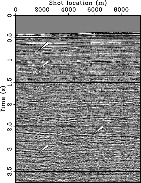
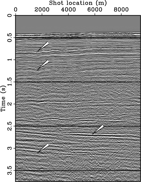
Figure 2(a) contains the common-offset section (at offset $200\,\mathrm{m}$ ) that we selected from a North Sea field dataset. Estimated primaries according to conventional SRME are plotted in Figure 2(b). Results where $\ell_2$ -matched filtering in the shot domain (Verschuur and Berkhout, 1997) is replaced by Bayesian thresholding (Saab et al., 2007) in the offset domain, are presented for a single offset in Figure 2(c), without scaling, and in Figure 2(d) with scaling. The scaled result is calculated for $\gamma =0.3$ . Juxtaposing the standard SRME and the curvelet-based results shows a removal of high-frequency clutter, which is in agreement with earlier findings reported in the literature. Moreover, primaries in the deeper part of the section (e.g. near the lower-two arrows in each plot) are much better preserved, compared to the standard-SRME result. Removal of the strong residual multiples in the shallow part, e.g. the first- and second-order water bottom multiples indicated by the arrows around $0.75$ and $1.20\, \mathrm{s}$ , is particularly exciting. Due to the unbalanced amplitudes of the predicted multiples, both standard SRME and non-adaptive Bayesian thresholding are not able to eliminate these events. Our adaptive method, however, successfully removes these events by virtue of the curvelet-domain scaling. Compared to non-adaptive thresholding, residual multiples are better suppressed, while our adaptive scheme also leads to at least similar, but often even better, overall continuity and amplitude preservation of the estimated primaries. For example, improvements are visible in the lower-left corner of the sections (between offsets $[0-2000]\,\mathrm{m}$ and times $[3.0-3.6]\,\mathrm{s})$ , where low-frequency multiple residuals are better suppressed after curvelet-domain matched filtering ( cf. Figure 2(c) and 2(d)), without deterioration of the primary energy. Finally, observe the improved recovery of primary energy at the lower arrow in Figure2(d), compared to the primary in Figure 2(c).

Figure2-a,Figure2-b,Figure2-c,Figure2-d
Figure 2. Adaptive curvelet-domain primary-multiple separation on real data. (a) Near-offset ( $200\,\mathrm{m}$ ) section for the total data plotted with automatic-gain control. (b) Estimate for the primaries, yielded by optimized one-term SRME computed with a windowed-matched filter. (c) Estimate for the primaries, computed by Bayesian iterative thresholding with a threshold defined by $\mathbf{t}=\vert\tensor{C}{\breve{\mathbf{s}}}_2\vert$ . (d) The same as (c) but now for the scaled (for $\gamma =0.3$ ) threshold, i.e., $\mathbf{t}=\vert\mathrm{diag}\{{\widetilde{\mathbf{w}}}\}\tensor{C}{\breve{\mathbf{s}}}_2\vert$ . Notice the improvement for the scaled estimate for the primaries, compared to the primaries yielded by SRME in (b) and by the Bayesian separation without scaling in (c).

Adaptive curvelet-domain primary-multiple separation