Adaptive curvelet-domain primary-multiple separation

Curvelet-domain matched filtering

Equation 2 lends itself to an inversion for the unknown scaling vector. As the true multiples are unknown, our formulation minimizes the least-squares mismatch between the total data and the predicted multiples. The following issues complicate the estimation of the scaling vector: (i) the undeterminedness of the forward model, due to the redundancy of the curvelet transform, i.e., $\tensor{C}\tensor{C}^T$ is rank deficient; (ii) the risk of overfitting the data, which leads to unwanted removal of primary energy, and (iii) the positivity requirement for the scaling vector. 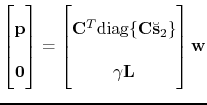To address issues (i-ii), the following augmented system of equations is formed that relates the unknown scaling vector $\mathbf{w}$ to the augmented data vector, $\mathbf{d}$ , i.e.,

$$\begin{bmatrix}\mathbf{p}\\ \mathbf{0} \end{bmatrix} = \begin{bma... ...\tensor{C}{\breve{\mathbf{s}}}_2\}\\ \gamma \tensor{L} \end{bmatrix} \mathbf{w}$$ (3)

or $\mathbf{d}=\tensor{F}_\gamma\mathbf{w}$ . The scaling vector is found by minimizing the functional

$$J_\gamma(\mathbf{z})=\frac{1}{2}\Vert\mathbf{d}-\tensor{F}_\gamma e^\mathbf{z}\Vert _2^2,$$ (4)

where the substitution of $\mathbf{w}=e^\mathbf{z}$ (with the exponentiation taken elementwise) guarantees positivity (issue (iii)) of the solution (Vogel, 2002). This formulation seeks a solution fitting the total data with a smoothness constraint imposed by the sharpening operator $\tensor{L}$ , which for each scale penalize fluctuations amongst neighboring curvelet coefficients in the space and angle directions (see Herrmann et al., 2007c, for a detailed description). The amount of smoothing is controlled by the parameter $\gamma$ . For increasing $\gamma$ , there is more emphasis on smoothness at the expense of overfitting the data (i.e., erroneously fitting the primaries). For a specific $\gamma$ , the penalty functional in Equation 4 is minimized with respect to the vector $\mathbf{z}$ with the limited-memory BFGS (Nocedal and Wright, 1999) with the gradient

$$\mathrm{grad}J(\mathbf{z})=\mathrm{diag}\{e^{\mathbf{z}}\}\big[\tensor{F}^T_\gamma\big(\tensor{F}_\gamma e^{\mathbf{z}}-\mathbf{d}\big)\big].$$ (5)

Ideally, the solution of the above optimization problem, ${\widetilde{\mathbf{z}}}=\mathop{\rm arg\,min}_\mathbf{z} J(\mathbf{z})$ , would, after applying the data-dependent scaling, yield the appropriate prediction for the multiples. Unfortunately, other phase and kinematic errors may interfere, rendering a separation based on the residual alone (as in SRME) ineffective, i.e., $\mathbf{p}-\tensor{C}^T\mathrm{diag}\{{\widetilde{\mathbf{w}}}\}\tensor{C}{\breve{\mathbf{s}}}_2$ with ${\widetilde{\mathbf{w}}}=e^{{\widetilde{\mathbf{z}}}}$ is an inaccurate estimate for the primaries. Robustness of threshold-based primary-multiple separation addresses this important issue and forms the second non-adaptive stage of our separation scheme.

Adaptive curvelet-domain primary-multiple separation