\[ \newcommand{\Pmat}{\mathbf{P}} \newcommand{\A}{\mathbf{A}} \newcommand{\q}{\mathbf{q}} \newcommand{\uvec}{\mathbf{u}} \newcommand{\post}{\text{post}} \newcommand{\rhopost}{\rho} \newcommand{\prior}{\text{prior}} \newcommand{\noise}{\text{noise}} \newcommand{\mis}{\text{mis}} \newcommand{\like}{\text{like}} \newcommand{\rholike}{\rho} \newcommand{\rholikepen}{{\rho}_{\text{like}}^{\text{pen}}} \newcommand{\overrholikepen}{\overline{\rho}_{\text{like}}^{\text{pen}}} \newcommand{\rhoprior}{\rho} \newcommand{\vvec}{\mathbf{v}} \newcommand{\obs}{\text{obs}} \newcommand{\dvec}{\mathbf{d}} \newcommand{\xvec}{\mathbf{x}} \newcommand{\Hmat}{\mathbf{H}} \newcommand{\Cmat}{\mathbf{C}} \newcommand{\g}{\mathbf{g}} \newcommand{\y}{\mathbf{y}} \newcommand{\dobs}{\mathbf{d}_{\text{obs}}} \newcommand{\F}{\mathbf{F}} \newcommand{\SIGMAN}{{\Gamma}_{\text{n}}} \newcommand{\SIGMANij}{_{i,j}{\Gamma}_{\text{noise}}} \newcommand{\SIGMAPDE}{{\Gamma}_{\text{pde}}} \newcommand{\SIGMAP}{{\Gamma}_{\text{p}}} \newcommand{\SIGMAU}{{\Gamma}_{\uvec}} \newcommand{\SIGMAS}{{\Gamma}_{\text{src}}} \newcommand{\SIGMAR}{{\Gamma}_{\text{rcv}}} \newcommand{\mvec}{\mathbf{m}} \newcommand{\Gmat}{\mathbf{G}} \newcommand{\Wmat}{\mathbf{W}} \newcommand{\Imat}{\mathbf{I}} \newcommand{\Lmat}{\mathbf{L}} \newcommand{\Llike}{\mathbf{L}_{\like}} \newcommand{\Lprior}{\mathbf{L}_{\text{prior}}} \newcommand{\Lpost}{\mathbf{L}_{\text{post}}} \newcommand{\Smat}{\mathbf{S}} \newcommand{\Rmat}{\mathbf{R}} \newcommand{\Mmat}{\mathbf{M}} \newcommand{\Jmat}{\mathbf{J}} \newcommand{\rvec}{\mathbf{r}} \newcommand{\nsrc}{n_{\text{src}}} \newcommand{\nrcv}{n_{\text{rcv}}} \newcommand{\nfreq}{n_{\text{freq}}} \newcommand{\ngrid}{n_{\text{grid}}} \newcommand{\ndata}{n_{\text{data}}} \newcommand{\nsmp}{n_{\text{smp}}} \newcommand{\mMAP}{\mathbf{m}_{\text{map}}} \newcommand{\Lmis}{\Lmat_{\text{mis}}} \newcommand{\nd}{n_{\text{data}}} \newcommand{\Hp}{\Hmat_{\text{prior}}} \newcommand{\fred}{f_\text{red}} \newcommand{\fpen}{f_\text{pen}} \newcommand{\Hlike}{\Hmat_{\text{like}}} \newcommand{\Hprior}{\Hmat_{\text{prior}}} \newcommand{\Hpost}{\Hmat_{\text{post}}} \renewcommand{\mp}{\tilde{\mvec}} \renewcommand{\SIGMAPDE}{\Gamma_{\text{PDE}}} \newcommand{\epssrc}{\epsilon_{\text{src}}} \newcommand{\epsrcv}{\epsilon_{\text{rcv}}} \]

Uncertainty quantification for inverse problems with a weak wave-equation constraint

Zhilong Fang¹*, Curt Da Silva¹, Rachel Kuske², and Felix J. Herrmann¹
¹Seismic Laboratory for Imaging and Modeling (SLIM), University of British Columbia
²Department of Mathematics, University of British Columbia

Abstract

In this work, we present a new posterior distribution to quantify uncertainties in solutions of wave-equation based inverse problems. By introducing an auxiliary variable for the wavefields, we weaken the strict wave-equation constraint used by conventional Bayesian approaches. With this weak constraint, the new posterior distribution is a bi-Gaussian distribution with respect to both model parameters and wavefields, which can be directly sampled by the Gibbs sampling method.

Introduction

In wave-equation based inverse problems, the goal is to infer the unknown model parameters from the observed data using the wave-equation as a constraint. Conventionally, the wave-equation is treated as a strict constraint in a Bayesian inverse problem. After eliminating this constraint, the problem involves the following forward modeling operator mapping model to predicted data: $\begin{equation} f(\mvec) = \Pmat\A(\mvec)^{-1}\q, \label{forward} \end{equation}$ where the vectors $\mvec \in \mathbb{R}^{\ngrid}$ and $\q \in \mathbb{C}^{\ngrid}$ represent the discretized $\ngrid$ -dimensional unknown model parameters and known source term, respectively. The matrix $\A \in \mathbb{C}^{\ngrid \times \ngrid}$ represents the discretized wave-equation operator and the operator $\Pmat \in \mathbb{R}^{\nrcv \times \ngrid}$ projects the solution of the wave equation $\uvec = \A(\mvec)^{-1}\q$ onto the $\nrcv$ receivers.

In the Bayesian framework, the solution of an inverse problem given observed data $\dvec$ is a posterior probability density function (PDF) $\rhopost(\mvec|\dvec)$ expressed as (Tarantola and Valette, 1982): $\begin{equation} \rhopost(\mvec|\dvec) \propto \rholike(\dvec|\mvec)\rhoprior(\mvec), \label{PostD} \end{equation}$ where the likelihood PDF $\rholike(\dvec|\mvec)$ describes the probability of observing data $\dvec$ given model parameters $\mvec$ and the prior PDF $\rhoprior(\mvec)$ describes one’s prior knowledge about the model parameters. Under the assumption that the noise in the data is Gaussian with zero mean and covariance matrix $\SIGMAN$ , and the prior distribution is also Gaussian with a mean model $\mp$ and covariance matrix $\SIGMAP$ , the posterior PDF can be written as: $\begin{equation} \rhopost(\mvec|\dvec) \propto \exp(-\frac{1}{2}(\|f(\mvec)-\dvec\|^{2}_{\SIGMAN^{-1}} + \|\mvec-\mp\|^{2}_{\SIGMAP^{-1}})). \label{PostD2} \end{equation}$ Due to the non-linear map $f(\mvec)$ and the high dimensionality of the model parameters ( $\ngrid \geq 10^5$ ), applying Markov chain Monte Carlo (McMC) methods to sample the posterior PDF $\eqref{PostD2}$ faces a difficult challenge of constructing a proposal PDF that provides a reasonable approximation of the target density with reasonable computational costs (Martin et al., 2012).

Posterior PDF with weak constraint

As the exact constraints $A(\mvec)\uvec = \q$ leads to the difficulty of studying the corresponding posterior PDF, we weaken the constraints and arrive at a more generic posterior PDF with an auxiliary variable – wavefields $\uvec$ as follows: $\begin{equation} \begin{aligned} \rhopost(\mvec,\uvec|\dvec) &\propto \rho_{1}(\dvec|\uvec)\rho_{2}(\uvec|\mvec)\rhoprior(\mvec), \text{ with } \\ \rho_{1}(\dvec|\uvec) &\propto \exp(-\frac{1}{2}\|\Pmat\uvec-\dvec\|^{2}_{\SIGMAN^{-1}}), \text{ and} \\ \rho_{2}(\uvec|\mvec) &\propto \exp(-\frac{\lambda^{2}}{2}\|\A(\mvec)\uvec-\q\|^2). \end{aligned} \label{PostDP} \end{equation}$ Here the penalty parameter $\lambda$ controls the trade off between the wave-equation and the data-fitting terms. As $\lambda$ grows, the wavefields are more tightly constrained by the wave equation. It is readily observed that the posterior PDF $\eqref{PostD}$ is a special case of the posterior PDF $\eqref{PostDP}$ with $\rho_{2}(\uvec|\mvec) = 1$ and $\A(\mvec)\uvec = \q$ .

The new posterior PDF $\eqref{PostDP}$ has two important properties. First, the conditional PDF $\rhopost(\uvec|\mvec,\dvec)$ of $\uvec$ on $\mvec$ is Gaussian. Second, if the matrix $\A(\mvec)$ linearly depends on $\mvec$ , the conditional PDF $\rhopost(\mvec|\uvec,\dvec)$ of $\mvec$ on $\uvec$ is also Gaussian. Therefore, the posterior PDF $\eqref{PostDP}$ is bi-Gaussian with respect to $\uvec$ and $\mvec$ .

Gibbs sampling

The bi-Gaussian property of the posterior PDF $\eqref{PostDP}$ provides a straight-forward intuition of applying Gibbs sampling method by alternatively drawing samples $\uvec$ and $\mvec$ from the conditional PDFs $\rhopost(\uvec|\mvec,\dvec)$ and $\rhopost(\mvec|\uvec,\dvec)$ . At the $k^{th}$ iteration of the Gibbs sampling, starting from the point $\mvec_{k}$ , the conditional PDF $\rhopost(\uvec|\mvec_{k},\dvec)$ $= \mathcal{N}(\overline{\uvec},\Hmat_{u}^{-1})$ with the Hessian matrix $\Hmat_{u}$ and the mean wavefields $\overline{\uvec}$ given by: $\begin{equation} \begin{aligned} \Hmat_{u} &= \Pmat^{\top}\SIGMAP^{-1}\Pmat + \lambda^2\A(\mvec_{k})^{\top}\A(\mvec_{k}), \\ \overline{\uvec} &= \Hmat_{u}^{-1}(\A(\mvec_{k})^{\top}\q+\Pmat^{\top}\SIGMAP^{-1}\dvec). \end{aligned} \label{OptU} \end{equation}$ To draw a sample $\uvec_{k+1} \sim \mathcal{N}(\overline{\uvec},\Hmat_{u}^{-1})$ , we first compute the Cholesky factorization of $\Hmat_{u} = \Lmat_{u}^{\top}\Lmat_{u}$ , where $\Lmat_{u}$ is an upper triangular matrix. Then we apply $\Lmat_{u}$ to compute $\overline{\uvec}$ and $\uvec_{k+1}$ by: $\begin{equation} \begin{aligned} \overline{\uvec} &= \Lmat_{u}^{-1}\Lmat_{u}^{-\top}(\A(\mvec_{k})^{\top}\q+\Pmat^{\top}\SIGMAP^{-1}\dvec), \\ \uvec_{k+1} &= \overline{\uvec} + \Lmat_{u}^{-1}\rvec_{u}, \rvec_{u} \sim \mathcal{N}(0,\mathbf{I}). \end{aligned} \label{Compuk1} \end{equation}$ With $\uvec_{k+1}$ , the conditional PDF $\rhopost(\mvec|\uvec_{k+1},\dvec)$ $=\mathcal{N}(\overline{\mvec},\Hmat_{m}^{-1})$ . The mean $\overline{\mvec} = \mvec_{k}-\Hmat_{m}^{-1}\g_{m}$ with gradient and Hessian expressed as: $\begin{equation} \begin{aligned} \g_{m} &= \Gmat^{\top}(\A(\mvec_{k})\uvec_{k+1} - \q) + \SIGMAP^{-1}(\mvec_{k}-\mp), \\ \Hmat_{m} &= \Gmat^{\top}\Gmat + \SIGMAP^{-1}, \end{aligned} \label{GandH} \end{equation}$ where $\Gmat = \frac{\partial \A(\mvec)\uvec_{k+1}}{\partial{\mvec}}$ is the sparse Jacobian matrix. The new sample $\mvec_{k+1}$ can be computed by: $\begin{equation} \mvec_{k+1} = \overline{\mvec} + \Lmat_{m}^{-1}\rvec_{m}, \rvec_{m} \sim \mathcal{N}(0,\mathbf{I}), \label{Sampm} \end{equation}$ where $\Lmat_{m} = \Hmat_{m}^{1/2}$ .

Numerical experiment

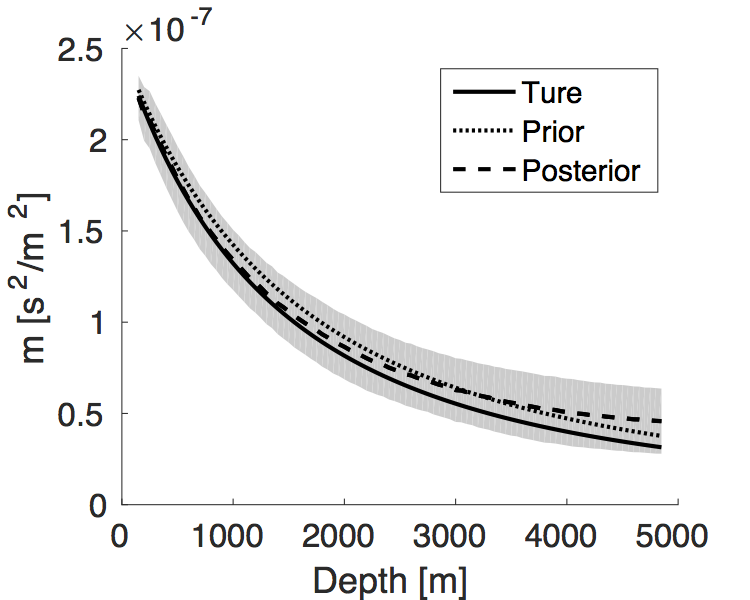
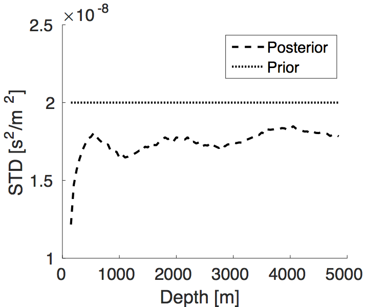
We apply our proposal method to an inverse problem constrained by the Helmholtz equation. We use single source, single frequency data to invert a 1D gridded squared slowness profile $m(z) = 1/(v_0 + \alpha z)^2$ for values $v_0 \, = \, 2000 \, \mathrm{m/s}$ and $\alpha \, = \, 0.75$ . We use frequency increments of $1 \, \mathrm{Hz}$ , a grid spacing of $50 \, \mathrm{m}$ , a maximum offset of $10000 \, \mathrm{m}$ , and a maximum depth of $5000 \, \mathrm{m}$ . Both source and receivers are located at the surface of the model. Gaussian noise with covariance matrix $\SIGMAN \, = \, \mathbf{I}$ is added to the data. The mean model of the prior distribution is selected to have $v_0 \, = \, 2000 \, \mathrm{m/s}$ and $\alpha \, = \, 0.65$ . The covariance matrix is set to $\SIGMAP = 2\times10^{-8}\mathbf{I}$ . We use the Gibbs sampling method to generate $$10^6$$ samples with $\lambda \, = \, 10^5$ . We compare the true model, the prior mean model, and the posterior mean model in Figure 1a, and the prior and posterior standard deviations (STD)in Figure 1b. The $90\%$ confidence interval of the posterior distribution is also shown in Figure 1a (gray background). Compared to the prior distribution, the posterior mean model has a smaller error in the shallow part but a larger error in the deep part. Meanwhile, the posterior STD in the shallow part has a larger decrease from the prior STD than that in the deep part. Both facts implies that data has a larger influence on the squared slowness in the shallow part than that in the deep part.

Conclusion

By weakening the wave-equation constraint in a controlled manner, we arrive at a novel formulation of posterior PDF for wave-equation inversion. This new posterior PDF is bi-Gaussian with respect to model parameters and wavefields. Numerical experiment demonstrate that this posterior PDF can be successfully and efficiently sampled by the Gibbs sampling method.

Acknowledgements

This research was carried out as part of the SINBAD project with the support of the member organizations of the SINBAD Consortium.

Martin, J., Wilcox, L. C., Burstedde, C., and Ghattas, O., 2012, A Stochastic Newton MCMC Method for Large-scale Statistical Inverse Problems with Application to Seismic Inversion: SIAM Journal on Scientific Computing, 34, A1460–A1487. Retrieved from http://epubs.siam.org/doi/abs/10.1137/110845598

Tarantola, A., and Valette, B., 1982, Inverse problems = quest for information: Journal of Geophysics, 50, 159–170.