Low-rank representation of subsurface extended image volumes with power iterations

Abstract

Full subsurface extended image volumes (EIVs) contain abundant information such as subsurface image gathers used in imaging, interpretation of rock properties or velocity analysis, but are expensive in term of computational cost and storage requirement due to their large size. Yet, due to their redundant information, monochromatic EIVs exhibit a low-rank structure that allows us to get a good approximation at a computational cost proportional to the rank \(k\) , while conventional techniques require at least the number of sources. Such low-rank factorized EIVs are computed thanks to the randomized singular values decomposition (SVD) algorithm. However, recent developments on low-rank approximations of EIVs raise two major questions. First, monochromatic EIVs rely on time-harmonic wave equation solvers, which do not scale well to realistic 3D models. Second, the rank of the monochromatic EIVs increases with the frequency, which yields increasing computational costs and storage. Here, we propose a construction approach based on a time-domain finite-difference wave-equation solver with time stepping, which is combined to power iteration schemes in the randomized SVD algorithm to accelerate the decay of the singular values. We compare the performances of simultaneous iterations, block-Krylov iterations and the original randomized SVD on the computation of the EIV for a small section of the Marmousi model. Then, we show further results on the full Marmousi model to validate our approach.

Introduction

Extended image volumes (EIVs) contain abundant subsurface information, including arbitrary subsurface gathers that are used not only for imaging, but also for the estimation of rock properties and velocity analysis in complex geological areas (Symes, 2008, Sava and Vasconcelos (2011)). Lots of comprehensive researches have been done to understand the behaviour and imaging principles of these gathers (Sava and Vasconcelos, 2011,Symes (2008)), which are achieved by taking multidimensional correlations of the source and receiver wavefields. With a kinematically correct velocity model, the EIVs’ energy will be mainly focused at zero offset. Migration-velocity analysis schemes use this property by minimizing an objective function that focuses the energy at zero offset (Sava and Biondi, 2004,Shen and Symes (2008)). However, these methods are impeded by large storage and computational costs that scale with the number of (horizontal) offsets and sources, respectively. Aside from these costs, which can become very large, these approaches almost exclusively work with horizontal subsurface offsets, which renders them less effective in areas with large geologic dips. In this latter situation, the practical compromise of limiting the number of subsurface points and horizontal subsurface-offset range may be inadequate.

Leeuwen and Herrmann (2012) addressed the issue of EIVs’ computational costs by showing that the expensive combination of a source loop and explicit computation of the cross correlation for each offset can be avoided by working with the “double wave equation” via probing, which involves the evaluation of only two partial differential equations (PDEs) for each subsurface point. While this probing approach makes it computationally feasible to compute full-subsurface offset EIV’s, three computational bottlenecks remain. First, the computation of each EIV involves a multi-dimensional convolution with the data. While computationally cheaper, the cost associated with this operation can still be significant. Da Silva et al. (2019) addressed this issue by using a low-rank tensor factorization technique with on-the-fly generation of shots. Second, the computational cost of forming full EIVs scale with the number of subsurface gridpoints, which is undesirable for most applications of EIVs. Third, so far this work was based on solutions of the time-harmonic wave equation, which scales poorly to 3D.

To overcome the second issue, Kumar et al. (2018) proposed to exploit the low-rank structure of monochromatic full subsurface EIVs, which can by virtue of its inherent redundancy be shown to have fast decaying singular values. To compute this low-rank matrix factorization, they used the randomized singular value decomposition (rSVD) introduced by Halko et al. (2011). With this technique, they were able to factor the double wave equation—i.e., EIVs for all subsurface points, in a low-rank form at a computational cost (PDE solves + multi-dimensional convolutions with the data) proportional to the rank \(k\). Because this rank is typically orders of magnitude smaller than the number of gridpoints and shots, we arrive at a formulation that is computationally feasible in terms of required storage, number of data passes (= convolution with the data), and PDE solves.

While this formulation based on the rSVD allowed us to manipulate the “unmanageable” large construct of full-subsurface offset gathers at all gridpoints, which is quadratic in the dimensionality of the image itself, two main challenges remain namely the use of time-domain wave-equation solvers and slow decay of singular values at the higher frequencies. We present solutions for both of these, which in principle allows us to compute subsurface-offset gathers at any (non-horizontal) offset and to carry out velocity continuation based on the invariance relationship presented by Kumar et al. (2018). Our construction is designed to scale to 3D. While we will incur one-time costs to carry out the low-rank factorization, the fact that we are low rank allows us to carry out subsequent manipulations, e.g. changing the velocity model, at costs that scale with the rank instead of the number of shots.

The paper is organized as follows: First, we present the equation for full EIVs and their low-rank representation using probing techniques. Next, we propose the modified low-rank representation based on time-domain finite-difference wave-equation solvers with time stepping. We then present our cost-effective computation of the low-rank representation with rSVD and power iterations. The latter allows us to deal with higher frequencies. We conclude by comparing the performance of conventional rSVD and power iteration schemes followed by an example from the Marmousi model.

Low-rank representation of extended image volumes

Full subsurface extended image volumes

According to Leeuwen et al. (2016), monochromatic extended image volumes (EIVs), containing subsurface offsets in all directions, can be formed as the outer product between the forward and adjoint wavefields: \[ \begin{equation} \mathbf{E}=\mathbf{H}^{-*}\mathbf{P}^T_r \mathbf{D} \mathbf{Q}^* \mathbf{P}_s \mathbf{H}^{-*}, \label{E_mono} \end{equation} \] where \(\mathbf{H}\) denotes the time-harmonic discretized Helmholtz operator. The matrix \(\mathbf{Q}\) of size \(N_s \times N_s\), with \(N_s\) the number of shots, contains discretized spatial sources. The matrix \(\mathbf{D}\), of size \(N_r \times N_s\) with \(N_r\) the number of receivers, contains reflection data with monochromatic shot records collected in its columns. Finally, the matrices \(\mathbf{P}_s\) and \(\mathbf{P}_r\) represent operators that restrict the wavefield to the source and receiver locations, respectively. We reserved the symbols \(^T\), \(^*\), and \(^{-*}\) to matrix transpose, conjugate transpose, and conjugate inverse.

Contrary to conventional subsurface-offset gathers, \(\mathbf{E}\) contains subsurface offsets in all directions. Given the fact that \(\mathbf{E}\) is a \(N_x\times N_x\) matrix with \(N_x\) being the number of grid points makes \(\mathbf{E}\) an object impossible to form and manipulate explicitly.

Low-rank representation using probing techniques

Instead of working with \(\mathbf{E}\) directly, we work with \(\mathbf{E}\) in low-rank factorized form (Kumar et al., 2018) that is accessible through probing (Leeuwen et al., 2017)—i.e., through matrix-free actions of \(\mathbf{E}\) on vectors that come at the cost of two wave-equation solves each. They justify this approach by arguing that the singular values of \(\mathbf{E}\) decay fast (Kumar et al., 2018) (its rank \(k\) is maximally \(n_s\)) so \(\mathbf{E}\) can be approximated accurately by a rank \(k\) matrix.

As long as we have access to matrix-free actions of \(\mathbf{E}\) and \(\mathbf{E}^*\), there are several ways to compute low-rank factorized \(\mathbf{E}\). We follow Kumar et al. (2018) and use the randomized SVD (rSVD) proposed by (Halko et al., 2011) and described in Algorithm 1. For a detailed explanation of this Algorithm, which costs \(4k\) PDE solves and data passes, we refer to Kumar et al. (2018).

Given the approximate low-rank factorization: \(\mathbf{E}\approx\mathbf{L}\mathbf{R}^*\) we have access to conventional zero-offset RTM images (see (Kumar et al., 2018)), to common image points (CIPs), and to images at different offsets.

Low-rank factorization in the time domain

While the proposed randomized SVD based framework can arguably circumvent the computational and memory bottleneck for 3D seismic data, monochromatic wave-equation solves do not scale well to 3D, which is problematic because step 2 and 4 of Algorithm 1 rely heavily on these solves. To address this issue, we proprose to use time-domain finite differences wave-equation based on the implementations provided by Devito (Lange et al., 2016) to factorize \(\mathbf{E}\) in its low-rank form. To incorporate time-domain solvers in our low-rank factorization, we probe with bandwidth limited vectors (white Gaussian noise for each subsurface point convolved with the temporal source waveform) as opposed to monochromatic Gaussian probing vectors in step 2 and 4 of Algorithm 1. We then carry out the multi-dimensional convolution with the data and the subsequent factorization in the Fourier domain. While we incur the cost of the Fourier transform, we are in this way able to use highly optimized finite-difference kernels for our wave simulations.

Following this procedure, we solve steps 2 and 4 with a time-domain solver. After Fourier transformation, we automatically get all the monochromatic probed results along frequencies, and we perform the sequent procedures of QR factorization and SVD monochromatically to the probed results.

Power iterations for randomized SVD

Although the time domain wave equation solvers outwit the computational limitations of solving the wave equations in 3D, we still face the issue of extending the low-rank factorization of EIV to higher frequencies. This is due to the increased spatial wave number content at these higher frequencies. As a result of that the singular values of EIVs decay more slowly at higher frequencies and we need to use higher ranks \(k\) to get reasonable quality EIVs. Unfortunately, this results in increasing computational costs negate the premise of our low-rank rSVD framework. To alleviate this problem, we propose to use power iterations (C. Musco and Musco, 2015), which use the fact that powers of EIV have faster decaying singular values while the singular vectors remain the same. While implementation of these power iterations increases the number of required wave equation solves, we only incur these additional costs once since the invariance relation will allow us to map the factors from one velocity model to another through velocity continuation at a cost proportional to the rank \(k\). We are now in a position to control these size of \(k\). We explain power-based rSVD as below:

Compared to original rSVD (Algorithm 1), rSVD with power iteration( Algorithm 2) (we mention as simultaneous iteration, SI) involves powers of the form \((\mathbf{E}\mathbf{E}^*)^q\). These terms come with extra costs in wave equation solves and data paths because we work with matrix-free products, and may also converge slowly as a function of \(q\) (C. Musco and Musco, 2015). To overcome this problem, we replace the expression for \(\mathbf{K}\) in Algorithm 2 line 2 by \(\mathbf{K}:=[\mathbf{E} \mathbf{W}, (\mathbf{E}\mathbf{E}^*) \mathbf{E} \mathbf{W}, \cdots, (\mathbf{E}\mathbf{E}^*)^q \mathbf{E} \mathbf{W}], \mathbf{K} \in \mathbb{C}^{N_x \times qk}\), resulting a faster convergence of \(q^2\) as recently proposed by C. Musco and Musco (2015).

Numerical results

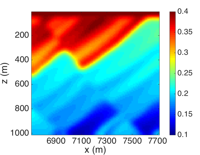
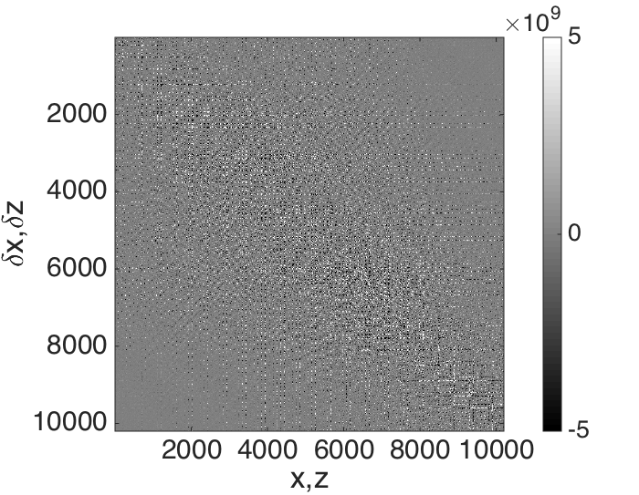
We now compare the performance of SI and BKI on the Marmousi model, with \(1100\times 314\) grid points respectively in x and z dimensions, discretized by \(10\text{m} \times 10\text{m}\). We consider \(550\) sources and receivers spreading over the model at depth \(15\text{m}\) with \(20\text{m}\) intervals. The data is generated by Born modeling trigged with Ricker wavelet centered at \(23 \text{Hz}\). To analyse the convergence of SI and BKI compared with rSVD, we first save out one explicit toy EIV at \(25\text{Hz}\) of one small section of \(100 \times 100\) grid points from Marmousi model, shown in Figure 1. The same exercise on the full Marmousi model would result into a matrix of order \(10^{12}\), which is too big to get stored explicitly. Then we will compare different image gathers, e.g. RTM images and CIPs from the low-rank represented EIV of Marmousi, recovered by the three algorithms: rSVD, SI and BKI.

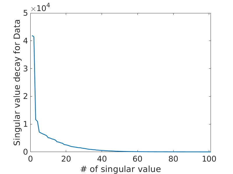
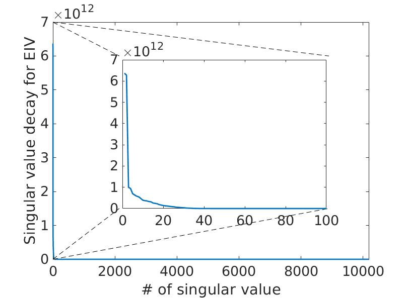
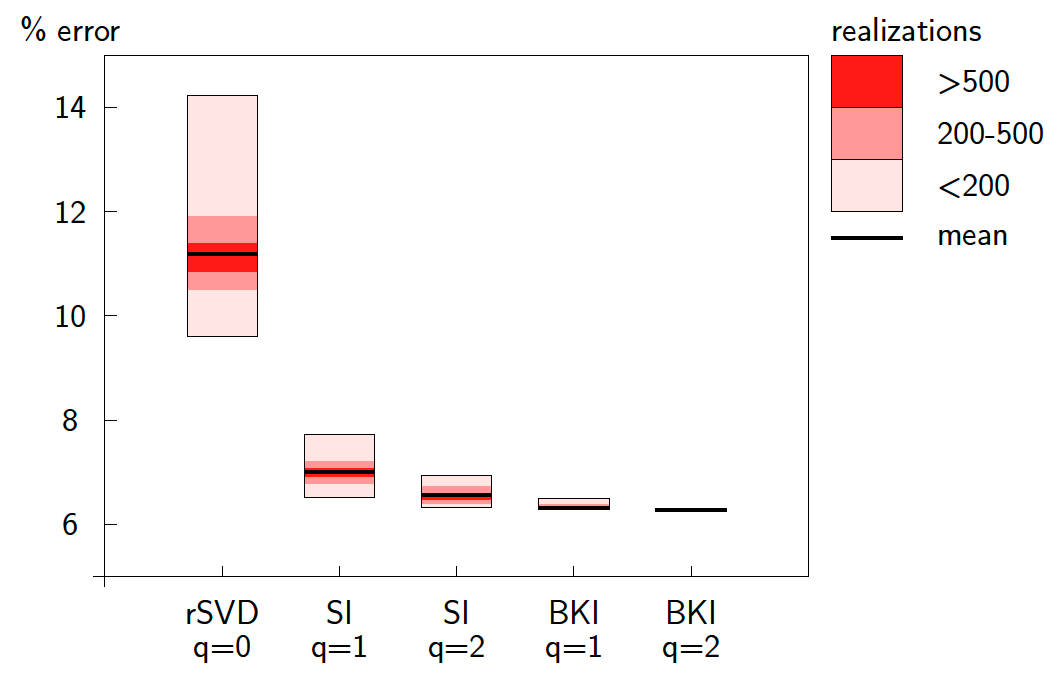
As shown in Figure 1(c), both the singular values of the EIV for the toy-example and of the corresponding data decay fast, the former decaying even faster than the latter. We recover this EIV with rSVD, SI and BKI with limited probing size \(r=14\), which corresponds to recover 95% of the energy of the EIV. To avoid the bias of randomness, we design statistical experiments to run \(1000\) times. In the experiment, we display the mean errors and the observed error ranges with realization for the three methods in Figure 2.

Figure 2 clearly shows that with \(r=14\), SI with \(q=1\) beats rSVD with much lower mean error. The error range of the former is narrower than that of the latter. And the realization colorbar shows clearly how many times we observe the errors in \(1000\) experiments. SI with \(q=2\) brings the error down a little compared with \(q=1\), but not significantly with respect to the additional required computational cost. BKI performs best among these three methods, offering the lowest mean errors and narrowest standard deviation. BKI with \(q=1\) works even better than SI with \(q=2\). The increase of the power for BKI doesn’t bring notable benefits since the mean errors don’t decrease obviously.

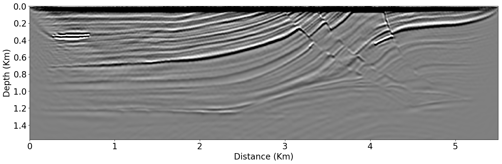
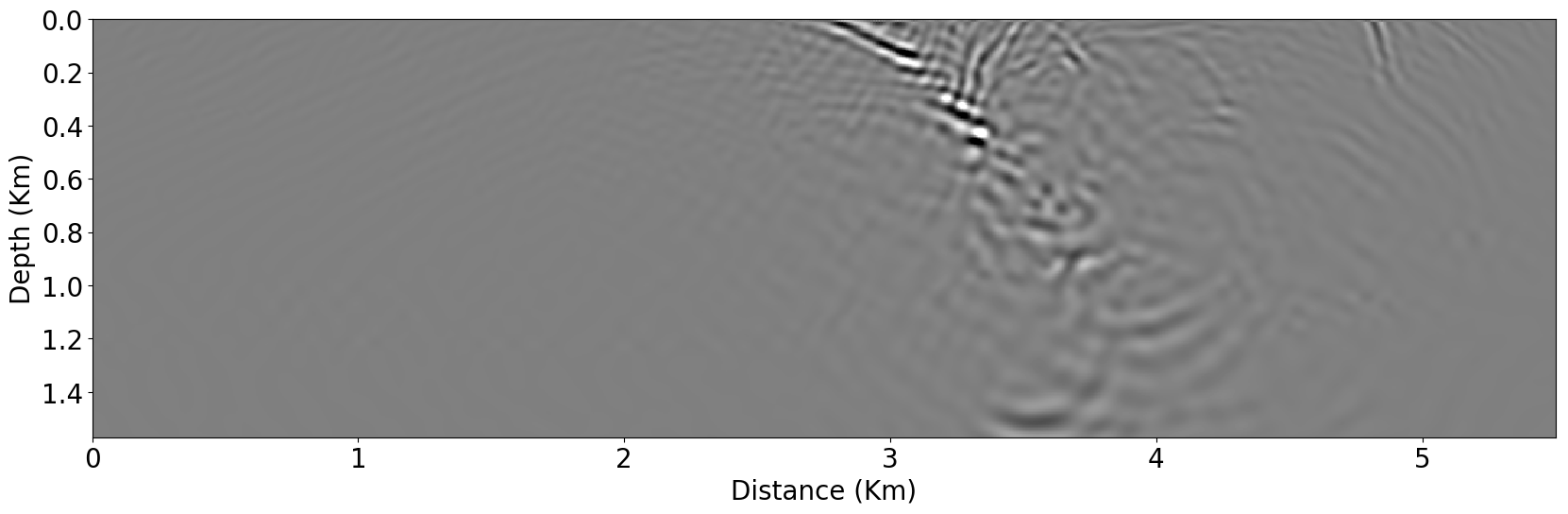
Based on the above observations from Figure 2 we only run power \(q\) up to \(1\) for SI and BKI for the Marmousi model. We now consider the full model and set the probing size \(r=25\) to recover the EIV. We expect the images extracted from EIV recovered by rSVD, shown in Figure 3(b) and Figure 4(b), contain good quality of low frequency components but with noise of high frequency components, compared to the corresponding exact images shown in Figure 3(a) and Figure 4(a). This is because the fixed probing size \(r=25\) is not large enough to recover the EIVs of higher frequencies whose singular values decay relatively slower. Figures 3(c) and 4(c) indicate that the corresponding images recovered by SI have better quality with higher frequency components recovered out than those of rSVD. Figures 3(d) and 4(d) recovered by BKI are better than those from SI. They demonstrate that BKI is the best for a fixed probing size \(r\).

Conclusion

Exploiting the low-rank structure of monochromatic full subsurface EIVs enables us to obtain an accurate approximation of the EIV at a reduced computational cost. This is possible by using the randomized SVD algorithm. The resulting computational cost is then proportional to the rank \(k\), which is much smaller than the number of shots or subsurface spatial grid points determining the cost of earlier techniques. However, this low-rank approach based on the time-harmonic wave equation did not prove will likely scale poorly in 3D. Therefore, we proposed to develop a low-rank approach to compute EIV based on the time-domain wave equation that involves all the frequencies at once. We also explored power iteration schemes in the rSVD algorithm, which accelerate the decay of the singular values without enlarging the rank \(k\). We compared the performances of simultaneous iterations (SI), block Krylov iterations (BKI) and rSVD on a small section of the Marmousi model, and then on the full model. Our results demonstrated that BKI proves to give a more accurate approximation with reasonable computational costs and storage requirements. We observed the results on extracted components, such as RTM images and CIP gathers, for the different variations of the iteration schemes.

Acknowledgements

This work was in part sponsored by the SINBAD project.