![]()
![]()
Abstract
Cloud computing has seen a large rise in popularity in recent years and is becoming a cost effective alternative to on-premise computing, with theoretically unlimited scalability. However, so far little progress has been made in adapting the cloud for high performance computing (HPC) tasks, such as seismic imaging and inversion. As the cloud does not provide the same type of fast and reliable connections as conventional HPC clusters, porting legacy codes developed for HPC environments to the cloud is ineffective and misses out on an opportunity to take advantage of new technologies presented by the cloud. We present a novel approach of bringing seismic imaging and inversion workflows to the cloud, which does not rely on a traditional HPC environment, but is based on serverless and event-driven computations. Computational resources are assigned dynamically in response to events, thus minimizing idle time and providing resilience to hardware failures. We test our workflow on two large-scale imaging examples and demonstrate that cost-effective HPC in the cloud is possible, but requires careful reconsiderations of how to bring software to the cloud.
Introduction
Reverse-time migration (RTM) (Baysal et al., 1983; Whitmore, 1983) and least-squares reverse-time migration (LS-RTM) (e.g. Valenciano, 2008) are among the most computationally challenging applications in scientific computing. RTM and LS-RTM are both demanding in terms of the number of necessary floating point operations for repeatedly solving large-scale wave-equations, as well as in terms of the memory required for storing the source wavefields. The traditional environment for running realistically sized seismic imaging workflows are high-performance computing (HPC) clusters, which are widely used in both academia and the oil and gas industry (e.g. Araya-Polo et al., 2009). However, due to the immense cost of acquiring and maintaining HPC clusters, cloud computing, with its pay-as-you-go pricing model and theoretically unlimited scalability, has evolved as a possible alternative to the traditional approach of HPC. Cloud computing and cloud services are already commonly used by many companies for hosting web content and databases, and clients include major companies such as Netflix or Philips. Increasingly, the customer list also includes companies from the O&G sector, such as Hess, Woodside, Shell or GE Oil & Gas (“AWS enterprise customer success stories,” 2019). According to case studies released by Amazon Web Services (AWS), the companies are using AWS for data storage and analytics, as well as marketing and cybersecurity.
While the cloud is becoming increasingly popular for general purpose computing tasks and data storage, it has so far fallen short of offering scalable solutions for HPC (Mauch et al., 2013). The straight-forward approach of connecting multiple compute instances of a cloud provider into a (virtual) cluster cannot offer the same stability, low latency and bandwidth as a traditional HPC cluster (Jackson et al., 2010). However, cloud computing offers a range of interesting novel technologies, such as object storage, event-driven computations, ElastiCache and spot pricing, which are not available in traditional HPC environments. These technologies offer new possibilities of addressing cost, computational challenges and bottlenecks in HPC and specifically seismic imaging, but they require a rethinking of how to design the corresponding workflows and software stacks, away from the classic client-server model.
In this work, we demonstrate a novel approach to HPC in the cloud, in which we take advantage of the aforementioned new technologies offered by cloud computing. Our workflow is based on a serverless computing architecture and is implemented on AWS, but the underlying programming model is applicable to other cloud providers as well. The workflow is generally usable for a variety of seismic imaging and inverse problems, such as LS-RTM or full-waveform inversion (FWI). The overall workflow is implemented using AWS Step Functions, while we use AWS Batch for massively parallel gradient computations and Lambda functions to sum the gradients of individual shots. We provide a general overview of the workflow and show its application to two synthetic datasets.
Workflow
We are interested in building workflows in the cloud for seismic inverse problems, such as FWI and LS-RTM. Mathematically, these problems correspond to solving optimization problems of the following form: \[ \begin{equation} \begin{split} \underset{\mathbf{m}}{\operatorname{minimize}} \hspace{0.2cm} \Phi(\mathbf{m}) = \sum_{i=1}^{n_s} ||\mathcal{F}(\mathbf{m})_i - \mathbf{d}_i ||^2_2, \\ \end{split} \label{objective} \end{equation} \] where \(\mathcal{F}(\mathbf{m})_i\) is a linear or non-linear partial differential operator, such as the acoustic forward modeling operator or the linearized Born scattering operator (e.g. Tarantola, 1984; Virieux and Operto, 2009). The vector \(\mathbf{m}\) denotes the unknown parameters such as a velocity model or a seismic image and \(\mathbf{d}_i\) are the observed shot records of the \(i^\text{th}\) source location. Instances of this problems such as FWI and LS-RTM are commonly addressed with gradient-based optimization algorithms such as (stochastic) gradient descent, the nonlinear conjugate gradient method, (Gauss-) Newton methods or sparsity-promoting techniques (e.g. Pratt, 1999; Felix J. Herrmann, 2010). The algorithms require that the gradient is computed for all (or a subset of) indices of the objective function, which is followed by summing the gradient parts and using it to update the model/image.
Conventionally, these steps are implemented as a single program, in which the work intensive parts such as the gradient computations are realized by distributing the workload to a range of workers using shared or distributed memory parallelism. Nodes or workers communicate via message passing (e.g. MPI) and rely on low latency and that connections are not interrupted within the duration of the program. These requirements pose a challenge in the cloud, where compute instances are oftentimes physically distributed over various locations and latency is several times larger than on HPC systems (Jackson et al., 2010). Furthermore, when using spot pricing, which can significantly reduce cost, instances are at risk of being shut down with a two minute warning at any given time (“AWS documentation,” 2019b).
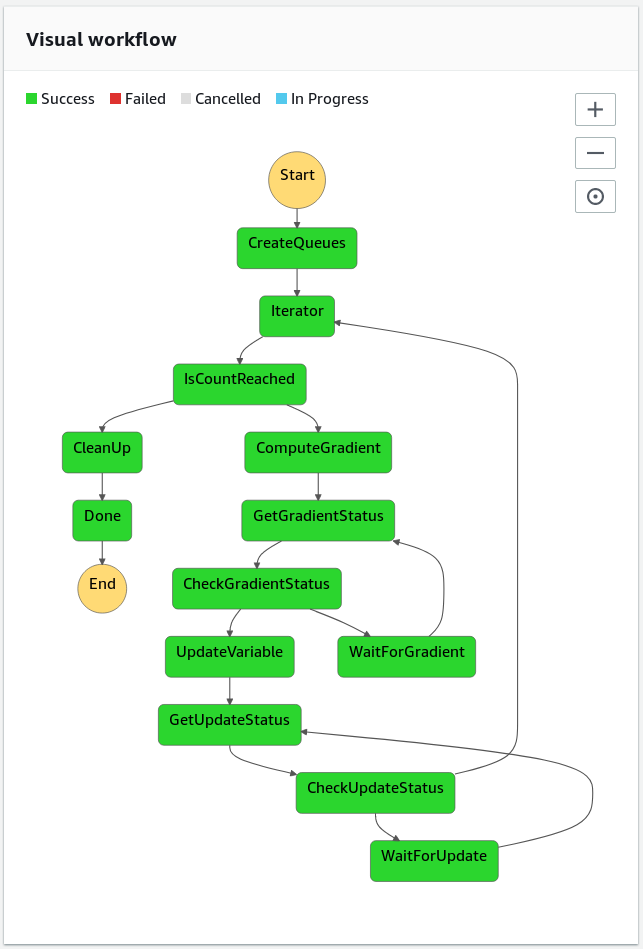
Rather than implementing our workflow for seismic inversion as a single program which runs on a virtual cluster, we compose our workflow of individual specialized AWS services. The workflow is serverless in the sense that no user process is required to stay alive during the entire execution time of the program. Individual tasks of the workflow such as computing or summing gradients are managed by AWS, including the handling of resilience in case of hardware failures. The basic structure of our workflow is implemented with AWS Step Functions, which allow to compose different AWS services into a serverless visual workflow (Figure 1). The design is inspired by a high-throughput genomics workflow as described in Friedman and Pizarro (2017). The workflow consists of an iterative loop, in which we subsequently compute the gradient of the objective function and update the optimization variable. The Iterator and IsCountReached tasks keep track of the iteration number and end the job after the final iteration number has been processed.
Computing gradients
The most work intensive part of seismic imaging and inversion workflows are the computation of the gradient of the objective function. This task involves solving a forward wave-equation to compute the predicted data and forward wavefields, as well as solving an adjoint wave-equation to compute the gradient. The gradient has to be computed for each source location, but the process of computing (individual) gradients is embarrassingly parallel.
AWS offers a service called AWS Batch that was exactly designed for this task, i.e. for running massively parallel batch computing jobs (“AWS documentation,” 2019a). The user submits individual jobs (i.e. computing a single gradient) to a job queue, while AWS Batch schedules the jobs and assigns the amount of computational resources for the duration required to run each job. As such, Batch does not only {handles>handle~} the responsibilities of a classic workload manager such as Slurm, but also chooses the optimal instance type for each job, which defines the amount of assigned storage, memory and number of CPUs. This flexibility is one of the strong points of cloud computing, as it gives user access to a wide range of instances that range from two core instances with \(4\) GB of memory to instances with up to \(96\) cores and \(768\) GB of memory.
AWS Batch runs individual jobs as Docker containers, which requires users to containerize the code for computing a single gradient as a Docker image. Generally, it is possible to add modeling codes of any programming language to a Docker container, but it is important to consider that user interfaces for the cloud (e.g. for writing results to buckets) exist only for high-level languages such as Python, but not for Fortran or C. In our workflow, we use the Julia Devito Inversion framework (JUDI) to compute individual gradients by solving the corresponding forward and adjoint wave-equations (Witte and Louboutin, 2018; P. A. Witte et al., 2019). JUDI is implemented in the Julia programming language and consists of symbolic operators and data containers that allow us to express modeling operations and gradients for seismic inversion in terms of linear algebra expression. For solving the underlying wave-equations, the framework uses Devito, a domain-specific language compiler for automatic code generation (Louboutin et al., 2018a; Luporini et al., 2018). Wave-equations in Devito are specified as symbolic Python expressions, from which optimized finite difference stencil code in C is generated and just-in-time compiled during run time.
In our workflow, AWS Batch is responsible for computing gradients for separate shot locations and the resulting files are stored as objects in AWS’s Simple Storage System (S3) (Figure 2). Since the gradients still need to be summed, each job also sends the filename of its result to a message queuing system (SQS), which in turn automatically invokes the gradient summation as soon as at least two files are available. The Batch jobs for computing the gradients itself are triggered by the ComputeGradient task in our Step Function workflow (Figure 1) and the jobs are automatically submitted to the Batch queue by an AWS Lambda function.
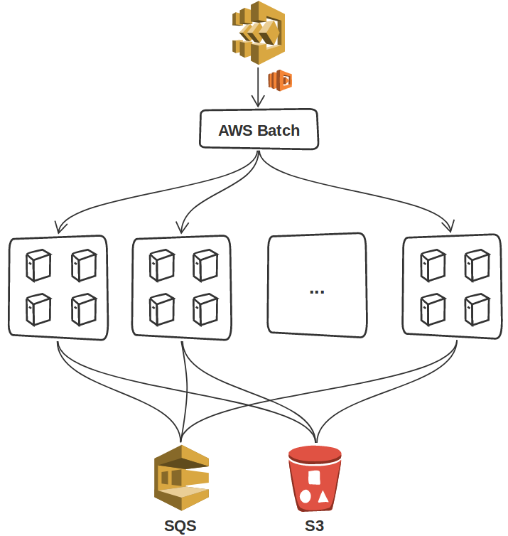
ComputeGradient task of the Step Functions. The results are written to an S3 bucket and each file name is send to an SQS queue. AWS Batch supports running each job on single or multiple compute instances.Gradient reduction
As AWS Batch is only designed to schedule and execute parallel jobs, but without the possibility to communicate between jobs, the summation of the individual gradients has to be implemented separately. For industry sized surveys, the number of summable gradients is typically very large (up to 1e6 gradients) and each gradient can be many gigabytes large. Since AWS Batch does not necessarily launch all jobs at the same time and the execution time per job may vary, results arrive in the S3 bucket at different times. We take advantage of this fact, by implementing an event-based gradient summation using AWS Lambda functions – serverless tasks that are launched in response to events. Each time a Batch worker computes a gradient and sends the resulting filename to our SQS queue, SQS triggers a Lambda function that reads up to \(10\) messages (i.e. filenames) from the queue (Figure 3). The Lambda function streams the files from S3, sums them and writes the summed gradient back to the bucket. The new file name is then added to the SQS queue and this process is repeated until all gradients have been computed and summed into a single file, at which point the Step Functions advance the workflow to the UpdateVariable task. This event-based approach ensures that the gradient reduction happens asynchronously (i.e. during the gradient computation), as soon as at least two files are available. Furthermore, the reduction happens in parallel, as multiple Lambda functions can be invoked at the same time.
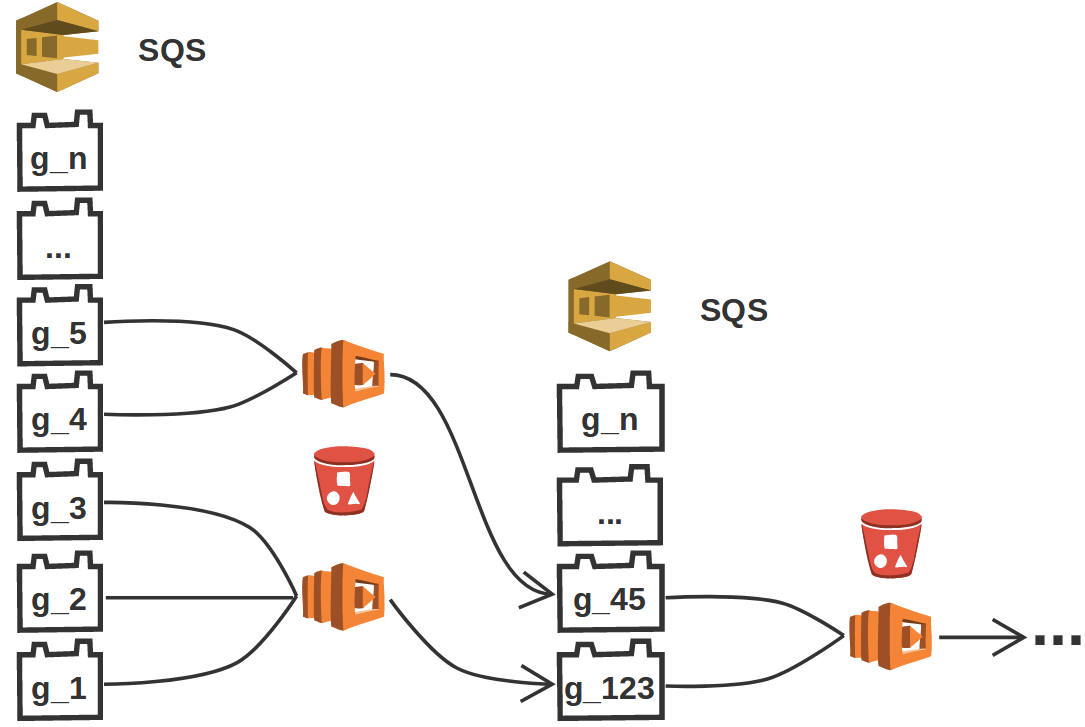
n gradients have been summed into a single file.Variable update
Once all gradients have been summed into a single file, the Step Functions progress the workflow to the subsequent task, in which we update our image or velocity model according to the update rule of a specific optimization algorithm. This can range from simple updates using multiplications with scalars (i.e. gradient descent), to more computationally demanding updates such as sparsity promotion, applying constraints or Gauss-Newton updates. Since Lambda functions are limited to \(3\) GB of memory and a maximum execution time of \(15\) minutes, we use AWS Batch for the more compute-heavy image/variable updates. The source code for the update is prepared as a Docker image and launched by the Step Function as a single job. The container reads the current image/model as well as the gradient from S3, updates the variables and writes it back to the bucket, which concludes a single iteration of our workflow.
Numerical examples
The workflow presented here is very general and can be applied to various seismic or non-seismic inverse problems with high compute and/or memory demands. The workflow can also be used to perform RTM by executing only a single iteration and omitting the variable update.
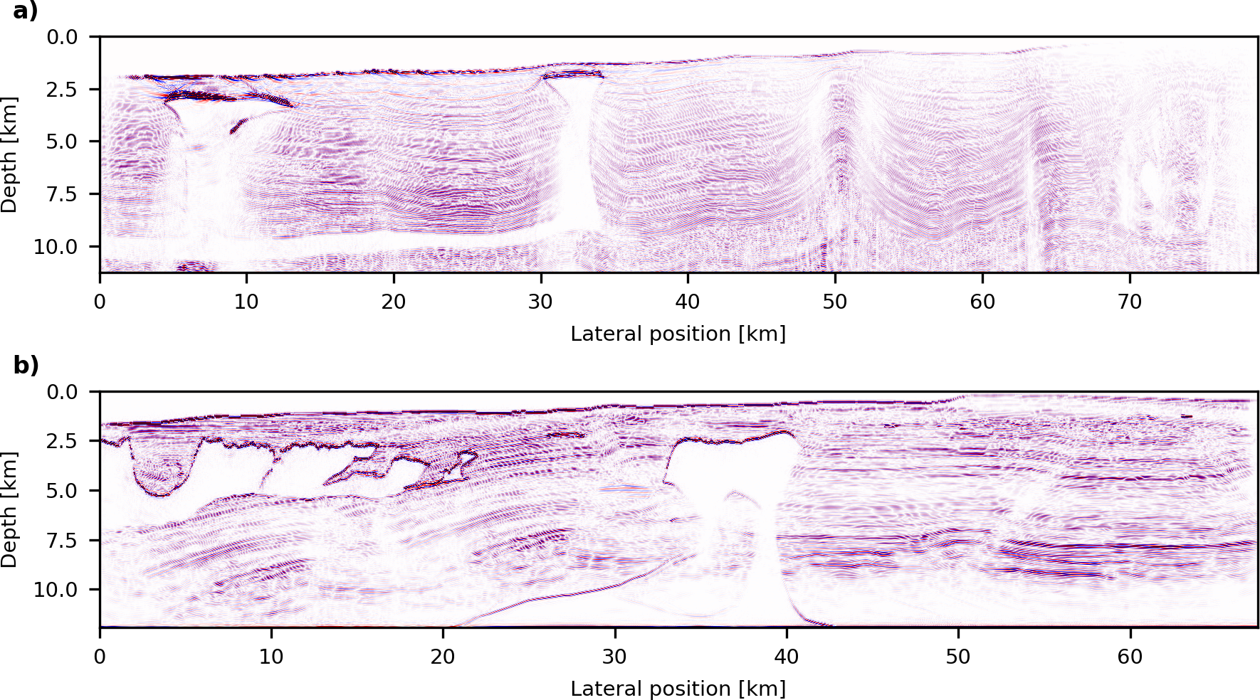
In our first numerical example, we use our workflow to perform RTM of the BP TTI 2007 dataset (Shah, 2007) (Figure 4 a). The model has a size of \(78.7\) by \(11.3\) km (\(12,596\) by \(1,801\) grid points) and the dataset consists of \(1641\) marine shot records. The workload of the Batch job for migrating the shot records consists of \(1641\) individual jobs, which are submitted to the Batch queue by the ComputeGradient task. We use a pseudo-acoustic formulation of the acoustic TTI wave-equation (Y. Zhang et al., 2011), with forward and adjoint equations that are implemented and solved with Devito (Louboutin et al., 2018b).
In this example, we demonstrate the possibility to use MPI-based domain decomposition in combination with AWS Batch, which is a feature that has been recently introduced by AWS. Multi-instance batch jobs allow us to use cheaper instances with less memory due to distributed memory parallelism. However, the downside of this approach is that AWS does not support spot pricing for multi-instance batch jobs, making this strategy comparatively more expensive. An overview of the job parameters, runtime and costs are provided in Table 1.
In our second example, we demonstrate an example of running an iterative imaging workflow using the BP Synthetic 2004 dataset (Billette and Brandsberg-Dahl, 2005) (Figure 4 b). Specifically, we perform \(20\) iterations of a sparsity-promoting LS-RTM workflow with shot subsampling, using the linearized Bregman method (Cai et al., 2009). The model has a size of \(67.4\) by \(11.9\) km (\(10,789\) by \(1,911\) grid points) and the dataset contains \(1348\) shot records. Each iteration involves computing the gradient for a subset of \(200\) randomly selected shots and updating the current image with curvelet-based sparsity-promotion (F.[] J.[] Herrmann et al., 2015). In comparison to our previous example, we only use a single AWS instance for each gradient computation, which allows us to use spot pricing. Even though this increases the runtime per gradient, as we have to use optimal checkpointing (Griewank and Walther, 2000), it reduces the cost per data pass by a factor \(3 - 4\) in comparison to on-demand pricing (Table 1).
| BP TTI 2007 | BP 2004 | |
|---|---|---|
| No. of shots | 1641 | 1348 |
| Instances/gradient | 6 | 1 |
| Instance type | m5.xlarge | r5.large |
| Runtime/gradient | 13.5 minutes | 45 minutes |
| On-demand price/gradient | 0.26 $ | 0.0945 $ |
| Spot price/gradient | N/A | 0.027 $ |
| On-demand price/data pass | 425.35 $ | 127.39 $ |
| Spot price/data pass | N/A | 35.99 $ |
Conclusions
Cloud-computing is a cost-effective alternative to conventional HPC with theoretically unlimited scalability. However, due to the fundamental differences of these computing environments, researchers have to rethink the way of designing software for HPC in the cloud, in a way that does not rely on the conventional client-server model. We introduce a serverless, event-driven workflow architecture, which makes use of AWS services to handle scheduling, cost effective resource assignment and resilience. Our event-driven approach ensures that resources are only allocated as long as they are needed and that hardware failures and interruptions do not bring down the whole workflow. We demonstrate that this allows us to run large-scale RTM and LS-RTM examples on AWS at very competitive costs.
Acknowledgements
We would like to thank to Geert Wenes from Amazon Web Services for his feedback and support. This research was carried out as part of the SINBAD II project with the support of the member organizations of the SINBAD Consortium.
References
Araya-Polo, M., Rubio, F., De la Cruz, R., Hanzich, M., Cela, J. M., and Scarpazza, D. P., 2009, 3D seismic imaging through reverse-time migration on homogeneous and heterogeneous multi-core processors: Scientific Programming, 17, 185–198.
AWS documentation: AWS Batch: 2019a, https://docs.aws.amazon.com/batch/latest/userguide/what-is-batch.html; Amazon Web Services User Guide. Retrieved March 19, 2019, from
AWS documentation: How spot instances work: 2019b, https://docs.aws.amazon.com/AWSEC2/latest/UserGuide/how-spot-instances-work.html; Amazon Web Services: User Guide for Linux Instances. Retrieved March 21, 2019, from
AWS enterprise customer success stories: 2019, https://aws.amazon.com/solutions/case-studies/enterprise; Amazon Web Services Case Studies. Retrieved March 19, 2019, from
Baysal, E., Kosloff, D. D., and Sherwood, J. W. C., 1983, Reverse time migration: GEOPHYSICS, 48, 1514–1524.
Billette, F., and Brandsberg-Dahl, S., 2005, The 2004 BP velocity benchmark.: In 67th Annual International Meeting, EAGE, Expanded Abstracts (p. B035). EAGE.
Cai, J.-F., Osher, S., and Shen, Z., 2009, Linearized Bregman iterations for compressed sensing: Mathematics of Computation, 78, 1515–1536.
Friedman, A., and Pizarro, A., 2017, Building high-throughput genomics batch workflows on AWS:. https://aws.amazon.com/blogs/compute/building-high-throughput-genomics-batch-workflows-on-aws-introduction-part-1-of-4/; AWS Compute Blog.
Griewank, A., and Walther, A., 2000, Algorithm 799: Revolve: An implementation of checkpointing for the reverse or adjoint mode of computational differentiation: Association for Computing Machinery (ACM) Transactions on Mathematical Software, 26, 19–45. doi:10.1145/347837.347846
Herrmann, F. J., 2010, Randomized sampling and sparsity: Getting more information from fewer samples: Geophysics, 75, WB173–WB187. doi:10.1190/1.3506147
Herrmann, F. J., Tu, N., and Esser, E., 2015, Fast “online” migration with Compressive Sensing: 77th Conference and Exhibition, EAGE, Expanded Abstracts. doi:10.3997/2214-4609.201412942
Jackson, K. R., Ramakrishnan, L., Muriki, K., Canon, S., Cholia, S., Shalf, J., … Wright, N. J., 2010, Performance analysis of high performance computing applications on the amazon web services cloud: In 2010 iEEE second international conference on cloud computing technology and science (pp. 159–168). IEEE.
Louboutin, M., Lange, M., Luporini, F., Kukreja, N., Witte, P. A., Herrmann, F. J., … Gorman, G. J., 2018a, Devito: An embedded domain-specific language for finite differences and geophysical exploration: ArXiv Preprints, arXiv:1808.01995. Retrieved from https://arxiv.org/abs/1808.01995
Louboutin, M., Witte, P. A., and Herrmann, F. J., 2018b, Effects of wrong adjoints for RTM in TTI media: SEG technical program expanded abstracts. doi:10.1190/segam2018-2996274.1
Luporini, F., Lange, M., Louboutin, M., Kukreja, N., Hückelheim, J., Yount, C., … Herrmann, F. J., 2018, Architecture and performance of Devito, a system for automated stencil computation: ArXiv preprints. Retrieved from https://arxiv.org/abs/1807.03032
Mauch, V., Kunze, M., and Hillenbrand, M., 2013, High performance cloud computing: Future Generation Computer Systems, 29, 1408–1416. doi:https://doi.org/10.1016/j.future.2012.03.011
Pratt, R. G., 1999, Seismic waveform inversion in the frequency domain, part 1: Theory and verification in a physical scale model: Geophysics, 64, 888–901. doi:10.1190/1.1444597
Shah, H., 2007, 2007 BP Anisotropic Velocity Benchmark:. https://wiki.seg.org/wiki/2007_BP_Anisotropic_Velocity_Benchmark; BP Exploration Operation Company Limited.
Tarantola, A., 1984, Inversion of seismic reflection data in the acoustic approximation: Geophysics, 49, 1259. doi:10.1190/1.1441754
Valenciano, A. A., 2008, Imaging by wave-equation inversion: PhD thesis,. Stanford University.
Virieux, J., and Operto, S., 2009, An overview of full-waveform inversion in exploration geophysics: GEOPHYSICS, 74, WCC127–WCC152. doi:10.1190/1.3238367
Whitmore, N. D., 1983, Iterative depth migration by backward time propagation: 1983 SEG Annual Meeting, Expanded Abstracts, 382–385.
Witte, P. A., and Louboutin, M., 2018, The Julia Devito Inversion Framework (JUDI):. https://github.com/slimgroup/JUDI.jl; GitHub.
Witte, P. A., Louboutin, M., Luporini, F., Kukreja, N., Lange, M., Gorman, G. J., and Herrmann, F. J., 2019, A large-scale framework for symbolic implementations of seismic inversion algorithms in Julia: Geophysics, 84, A31–V183.
Zhang, Y., Zhang, H., and Zhang, G., 2011, A stable TTI reverse time migration and its implementation: Geophysics, 76, WA3–WA11. doi:10.1190/1.3554411