A dual formulation for time-domain wavefield reconstruction inversion

Gabrio Rizzuti¹, Mathias Louboutin¹, Rongrong Wang², Emmanouil Daskalakis³, and Felix J. Herrmann^1
1 Georgia Institute of Technology,
² Michigan State University,
³ University of British Columbia, now Vancouver Community College

Abstract

We illustrate a dual formulation for full-waveform inversion potentially apt to large 3-D problems. It is based on the optimization of the wave equation compliance, under the constraint of data misfit not exceeding a prescribed noise level. In the Lagrangian formulation, model and wavefield state variables are complemented with multipliers having the same dimension of data (“dual data” variables). Analogously to classical wavefield reconstruction inversion, the wavefield unknowns can be projected out in closed form, by solving a version of the augmented wave equation. This leads to a saddle-point problem whose variables are only model and dual data. As such, this formulation represents a model extension, and is potentially robust against local minima. The classical downsides of model extension methods and wavefield reconstruction inversion are here effectively mitigated: storage of the dual variables is affordable, the augmented wave equation is amenable to time-marching finite-difference schemes, and no continuation strategy for penalty parameters is needed, with the prospect of 3-D applications.

Introduction

Full-Waveform Inversion (FWI) can be cast as a constrained optimization problem: \[ \begin{equation} \min_{\mathbf{m},\mathbf{u}}\ \frac{1}{2}||\mathbf{d}-R\,\mathbf{u}||^2\quad\mathrm{subject\ to}\quad A(\mathbf{m})\,\mathbf{u}=\mathbf{q}. \label{eqPDEconstraint} \end{equation} \] We aim at the optimal least-squares data misfit under the wave-equation constraint (Biros and Ghattas, 2005; Grote et al., 2011; Leeuwen and Herrmann, 2013; Peters et al., 2014). Here, the unknowns are represented by \(\mathbf{m}\), collecting model parameters (e.g., the acoustic squared slowness), and \(\mathbf{u}\), the pressure wavefield defined for every source and time or frequency. The operator \(R\) restricts \(\mathbf{u}\) to the receiver positions, where it is compared to the collected data \(\mathbf{d}\). The wave equation is summarized by the linear operator \(A(\mathbf{m})\) (dependent on \(\mathbf{m}\)) and right hand sides \(\mathbf{q}\) (typically point sources).

The traditional approach to the problem in eq. \(\eqref{eqPDEconstraint}\) is based on the exact solution of the wave equation: \[ \begin{equation} A(\mathbf{m})\,\mathbf{u}=\mathbf{q}, \label{eqwaveq} \end{equation} \] which leads to the reduced FWI objective \[ \begin{equation} \min_\mathbf{m}\,\frac{1}{2}||\mathbf{d}-F(\mathbf{m})\,\mathbf{q}||^2,\quad F(\mathbf{m})=R\,A(\mathbf{m})^{-1} \label{eqFWI} \end{equation} \] (Tarantola and Valette, 1982). Computationally, the fundamental challenge for FWI is the need for efficient solvers for the wave equation \(\eqref{eqwaveq}\). For large problems, time-domain solvers currently scale better than their frequency-domain counterparts when explicit time-marching schemes are employed (performances are comparable only when abundant compute cores are available, Knibbe et al., 2016). Also, note that the evaluation and gradient computation for the objective in eq. \(\eqref{eqFWI}\) do not require the solution wavefields to be stored for every source and time/frequency (e.g., see for a checkpointing strategy in time domain W. W. Symes, 2007). Time-domain FWI has been proven feasible for industrial-scale 3-D applications.

A notorious issue with FWI is its liability to local minima (Virieux and Operto, 2009). Recently, many model extension methods have been proposed as a way to circumvent the problem, by complementing the model parameter search space with physically/mathematically-motivated dummy variables in order to achieve better data fit. At the same time, the consistency with the original problem need be promoted with ad-hoc regularization (W. W. Symes, 2008; Biondi and Almomin, 2014; Leeuwen and Herrmann, 2013; Warner and Guasch, 2016; Wu and Alkhalifah, 2015; Huang et al., 2017; Aghamiry et al., 2019). The space extension, however, must be chosen carefully in order to control the well-posedness of the problem, and the memory footprint needed to store the additional variables.

An instance of these methods particularly relevant for this work is based on the Lagrangian formulation of eq. \(\eqref{eqPDEconstraint}\): \[ \begin{equation} \max_\mathbf{v}\ \min_{\mathbf{m},\mathbf{u}}\ \frac{1}{2}||\mathbf{d}-R\,\mathbf{u}||^2+\langle \mathbf{v},\mathbf{q}-A(\mathbf{m})\,\mathbf{u}\rangle \label{eqfullSpaceLagr} \end{equation} \] (\(\langle\cdot,\cdot\rangle\) denoting the Euclidean inner product). The multipliers \(\mathbf{v}\) belong to the same functional space as the wavefields \(\mathbf{u}\). Furthermore, the evaluation and gradient computation in eq. \(\eqref{eqfullSpaceLagr}\) do not require the solution of the wave equation (Haber et al., 2000). However, the storage of wavefields and dual variables for every source and time sample/frequency is unfeasible in 3-D (in the order of petabytes for a model of 1000\(^3\) grid points and data acquired in time domain with sparse source coverage).

The penalty method approach allows to avoid the multiplier estimation by substituting \(\mathbf{v}=\lambda^2\,(\mathbf{q}-A(\mathbf{m})\,\mathbf{u})/2\) in eq. \(\eqref{eqfullSpaceLagr}\), given a certain weight \(\lambda\), yielding \[ \begin{equation} \min_{\mathbf{m},\mathbf{u}}\ \frac{1}{2}||\mathbf{d}-R\,\mathbf{u}||^2+\frac{\phantom{^2}\lambda^2}{2}||\mathbf{q}-A(\mathbf{m})\,\mathbf{u}||^2 \label{eqpenalty} \end{equation} \] (Berg and Kleinman, 1997; Leeuwen and Herrmann, 2013). This comes at the cost of perturbing the original problem, and a rigorous solution should involve a continuation strategy for \(\lambda\to\infty\). In the Wavefield Reconstruction Inversion scheme (WRI, Leeuwen and Herrmann, 2013), a variable projection scheme is employed (Golub and Pereyra, 2003), which leads to the augmented wave equation: \[ \begin{equation} \begin{split} \begin{bmatrix} R\\ \lambda A(\mathbf{m}) \end{bmatrix} \bar{\mathbf{u}}= \begin{bmatrix} \mathbf{d}\\ \lambda \mathbf{q} \end{bmatrix}, \end{split} \label{eqaugwaveq} \end{equation} \] to be solved in a minimum-norm sense. Although this procedure eliminates the need for simultaneous wavefield storage, it requires the solution of a wave-equation related system which is not easily tractable in the time domain (but refer to C. Wang et al., 2016 for a workaround), and does not scale better than the conventional wave equation in frequency domain (although, see Leeuwen and Herrmann, 2014; Peters et al., 2015).

In this paper, we are interested in combining a model-extension approach, in order to leverage on local search optimization schemes with a mitigated risk against spurious minima, and the computational convenience of reduced approaches, especially with respect to the availability of time-marching solvers for the wave equation (or augmented version thereof). The model extension need be feasible, i.e. the additional variables should easily fit in memory.

Theory

Our proposal starts from the denoising version of eq. \(\eqref{eqPDEconstraint}\), based on a data-misfit constraint (R. Wang and Herrmann, 2017): \[ \begin{equation} \min_{\mathbf{m},\mathbf{u}}\ \frac{1}{2}||\mathbf{q}-A(\mathbf{m})\,\mathbf{u}||^2\quad\mathrm{s.t.}\quad ||\mathbf{d}-R\,\mathbf{u}||\le\varepsilon. \label{eqdenoising} \end{equation} \] Here, \(\varepsilon\) is a given noise level. Analogously to eq. \(\eqref{eqfullSpaceLagr}\), the associated Lagrangian problem is \[ \begin{equation} \begin{split} & \max_\mathbf{y}\ \min_{\mathbf{m}, \mathbf{u}}\ \mathcal{L}(\mathbf{m},\mathbf{u},\mathbf{y}),\\ & \mathcal{L}(\mathbf{m},\mathbf{u},\mathbf{y})=\frac{1}{2}||\mathbf{q}-A(\mathbf{m})\,\mathbf{u}||^2+\langle \mathbf{y},\mathbf{d}-R\,\mathbf{u}\rangle-\varepsilon||\mathbf{y}||. \end{split} \label{eqlagr} \end{equation} \] It can be verified that \(\max_{\mathbf{y}}\ \langle\mathbf{y},\mathbf{d}-R\,\mathbf{u}\rangle-\varepsilon||\mathbf{y}||\) is the indicator function on the constraint set \(C_{\varepsilon}=\{\mathbf{d}:||\mathbf{d}-R\,\mathbf{u}||\le\varepsilon\}\).

The wavefield variables \(\mathbf{u}\) are eliminated from eq. \(\eqref{eqlagr}\) by solving the following augmented wave equation: \[ \begin{equation} A(\mathbf{m})\,\bar{\mathbf{u}}=\mathbf{q}+F(\mathbf{m})^*\,\mathbf{y} \label{eqaugwaveq2} \end{equation} \] (\(^*\) denotes the adjoint operator). Here, the backpropagated dual data \(\mathbf{y}\) acts as an additional volumetric source for \(\bar{\mathbf{u}}\). The choice \(\mathbf{y}=\mathbf{0}\) restores the conventional wave equation.

Substituting the expression in eq. \(\eqref{eqaugwaveq2}\) in eq. \(\eqref{eqlagr}\) leads to the reduced saddle-point problem: \[ \begin{equation} \begin{split} & \max_{\mathbf{y}}\ \min_{\mathbf{m}}\ \bar{\mathcal{L}}(\mathbf{m},\mathbf{y}),\\ & \bar{\mathcal{L}}(\mathbf{m},\mathbf{y})=-\frac{1}{2}||F(\mathbf{m})^*\,\mathbf{y}||^2+\langle \mathbf{y},\mathbf{d}-F(\mathbf{m})\,\mathbf{q}\rangle-\varepsilon||\mathbf{y}||. \end{split} \label{eqlagrred} \end{equation} \] The gradients of \(\bar{\mathcal{L}}\) with respect to \(\mathbf{m}\) and \(\mathbf{y}\), when \(\mathbf{y}\neq\mathbf{0}\), are: \[ \begin{equation} \begin{split} & \nabla_{\mathbf{m}}\bar{\mathcal{L}}=-\mathrm{D}F[\mathbf{m},\mathbf{q}+F(\mathbf{m})^*\,\mathbf{y}]^*\,\mathbf{y},\\ & \nabla_{\mathbf{y}}\bar{\mathcal{L}}=\mathbf{d}-F(\mathbf{m})\,(\mathbf{q}+F(\mathbf{m})^*\,\mathbf{y})-\varepsilon\,\mathbf{y}/||\mathbf{y}||. \end{split} \label{eqgrad} \end{equation} \] When \(\mathbf{y}=\mathbf{0}\), a subgradient of \(\bar{\mathcal{L}}\) is \(\nabla_{\mathbf{y}}\bar{\mathcal{L}}=\mathbf{d}-F(\mathbf{m})\,\mathbf{q}\). Here \(\mathrm{D}F[\mathbf{m},\mathbf{f}]\) denotes the Jacobian of the forward map \(F(\mathbf{m})\,\mathbf{f}\) with respect to \(\mathbf{m}\). Note that \(\nabla_{\mathbf{m}}\bar{\mathcal{L}}\) is similar to the gradient of conventional FWI, since it is computed by the zero-lag cross-correlation of the forward wavefield \(\bar{\mathbf{u}}\) in eq. \(\eqref{eqaugwaveq2}\) and the backpropagated (dual) data wavefield \(F(\mathbf{m})^*\,\mathbf{y}\). The gradient \(\nabla_{\mathbf{y}}\bar{\mathcal{L}}\) is simply the data residual of the augmented wavefield \(\bar{\mathbf{u}}\), relaxed by the corrective term \(\varepsilon\,\mathbf{y}/||\mathbf{y}||\).

The augmented system in eq. \(\eqref{eqaugwaveq2}\) is determined (for a fixed \(\mathbf{y}\)), and is amenable to time-domain methods. The same holds true for the evaluation and gradient computation of \(\bar{\mathcal{L}}\). Also, the dual variable \(\mathbf{y}\), having the same dimension of the data \(\mathbf{d}\), can be conveniently stored in memory, which makes the optimization of \(\bar{\mathcal{L}}\) affordable.

Possible optimization strategies for the problem in eq. \(\eqref{eqlagrred}\) are alternating updates (as in the alternating direction method of multipliers, Boyd et al., 2011; Aghamiry et al., 2019) or quasi-Newton methods (as L-BFGS, Nocedal and Wright, 2006). Given an initial background model \(\mathbf{m}_0\), a natural starting guess for \(\mathbf{y}\) is a scaled version of the data residual \(\mathbf{y}_0\propto \mathbf{r}_0=\mathbf{d}-F(\mathbf{m}_0)\,\mathbf{q}\). The scaling factor must be chosen carefully, as it weights the relative contribution of \(\mathbf{y}\) in the augmented wavefield, with respect to the physical source \(\mathbf{q}\). In this respect, its role is akin to the weighting parameter \(\lambda\) in WRI (see eq. \(\eqref{eqaugwaveq}\)). However, due to the underlying Lagrangian formulation, it can be promptly adapted to any particular pair \((\mathbf{m},\mathbf{y})\). The optimal scaling factor \(\arg\max_{\alpha}\bar{\mathcal{L}}(\mathbf{m},\alpha\,\mathbf{y})\) is calculated explicitly by: \[ \begin{equation} \alpha(\mathbf{m},\mathbf{y})=\left\{ \begin{split} & \mathrm{sign}\langle \mathbf{y}, \mathbf{r}\rangle\frac{|\langle \mathbf{y}, \mathbf{r}\rangle|-\varepsilon\,||\mathbf{y}||}{||F(\mathbf{m})^*\,\mathbf{y}||^2}, & |\langle \mathbf{y}, \mathbf{r}\rangle|\ge\varepsilon\,||\mathbf{y}||,\\ & 0, & \mathrm{otherwise},\\ \end{split} \right.\ \label{eqalpha} \end{equation} \] where \(\mathbf{r}=\mathbf{d}-F(\mathbf{m})\,\mathbf{q}\) is the data residual. Plugging this formula in eq. \(\eqref{eqlagrred}\) produces a scale-invariant Lagrangian \(\bar{\bar{\mathcal{L}}}(\mathbf{m},\mathbf{y}):=\bar{\mathcal{L}}(\mathbf{m},\alpha\,\mathbf{y})\): \[ \begin{equation} \bar{\bar{\mathcal{L}}}(\mathbf{m},\mathbf{y})=\left\{ \begin{split} & \frac{1}{2}(|\langle\hat{\mathbf{y}},\mathbf{r}\rangle|-\varepsilon\,||\hat{\mathbf{y}}||)^2, & |\langle\hat{\mathbf{y}}, \mathbf{r}\rangle|\ge\varepsilon\,||\hat{\mathbf{y}}||,\\ & 0, & \mathrm{otherwise},\\ \end{split} \right. \label{eqlagrredscal} \end{equation} \] where \(\hat{\mathbf{y}}=\mathbf{y}/||F(\mathbf{m})^*\,\mathbf{y}||\). Since \(\bar{\bar{\mathcal{L}}}\) has been obtained from a variable projection scheme, the corresponding gradient expression follows directly from eq. \(\eqref{eqgrad}\): \[ \begin{equation} \begin{split} & \nabla_{\mathbf{m}}\bar{\bar{\mathcal{L}}}(\mathbf{m},\mathbf{y})=\nabla_{\mathbf{m}}\bar{\mathcal{L}}(\mathbf{m},\alpha\,\mathbf{y}),\\ & \nabla_{\mathbf{y}}\bar{\bar{\mathcal{L}}}(\mathbf{m},\mathbf{y})=\alpha\nabla_{\mathbf{y}}\bar{\mathcal{L}}(\mathbf{m},\alpha\,\mathbf{y}).\\ \end{split} \label{eqgradscal} \end{equation} \] Eq. \(\eqref{eqlagrredscal}\) offers a simple geometric interpretation of how the variables \(\mathbf{m},\mathbf{y}\) are optimized, here seen as vectors in the Euclidean space. The maximization of \(\bar{\bar{\mathcal{L}}}\) with respect to \(\mathbf{y}\) results in an updated \(\hat{\mathbf{y}}\) more aligned with respect to the residual \(\mathbf{r}\). Note that the norm of \(\hat{\mathbf{y}}\) remains bounded from above and below due to the (quasi-)normalization induced by the factor \(c_1(\mathbf{m})||\mathbf{y}||\le||F(\mathbf{m})^*\,\mathbf{y}||\le c_2(\mathbf{m})||\mathbf{y}||\), with \(c_1(\mathbf{m})>0\), \(c_2(\mathbf{m})>0\). The minimization of \(\bar{\bar{\mathcal{L}}}\) with respect to \(\mathbf{m}\), instead, will reduce the length of the projection of the residual \(\mathbf{r}\) on \(\hat{\mathbf{y}}\), by decreasing the norm of \(\mathbf{r}\) and/or by making \(\mathbf{r}\) more orthogonal to \(\hat{\mathbf{y}}\) (up to a tolerance governed by \(\varepsilon\)).

We conclude this section with a brief observation on the computational demands for the dual formulation. We already stressed the memory complexity advantages over general extended modeling methods, and the unfeasibility of a rigorous time-domain approach for WRI. For the sake of a comparison with conventional FWI, we consider the cost for the solution of the wave equation as the basic working unit. The gradient computation in eq. \(\eqref{eqgrad}\) requires the same work of FWI: that is, two working units for forward and backward propagation. However, with an alternating update procedure, the overall update for \(\mathbf{m}\) requires an intermediate \(\mathbf{y}\) estimation, which results in twice as much the cost needed for the update of \(\mathbf{m}\) for FWI.

Examples

In this section we present some examples that illustrates the main theoretical features of the method.

Augmented wave equation

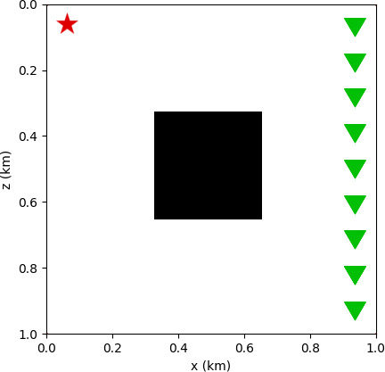
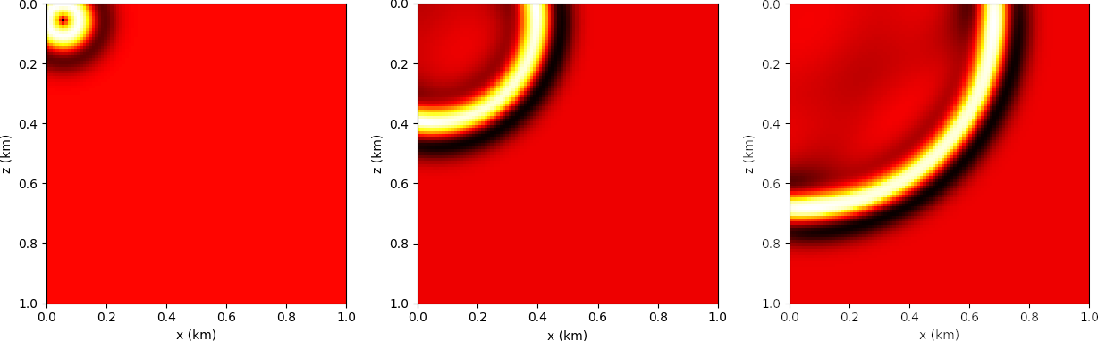
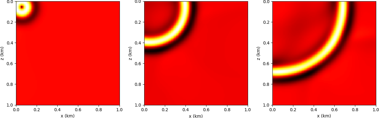
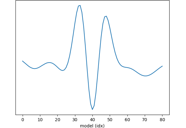
In Figures 1 and 2, we demonstrate the difference between the solution of the conventional wave equation \(\eqref{eqwaveq}\) and the augmented wave equation \(\eqref{eqaugwaveq2}\). In Figure 2, the difference between wavefield snapshots reveals the effect of the dual variable \(\mathbf{y}\), here chosen to be the data residual between perturbed and homogeneous models (Figure 1). The variable \(\mathbf{y}\) acts as a secondary source (cf. eq. \(\eqref{eqaugwaveq2}\)). Note that both wavefields propagate through an homogeneous medium, and there is no physical scattering effect due to the perturbation. The difference is entirely due to the backpropagation of \(\mathbf{y}\).

Lagrangian landscape

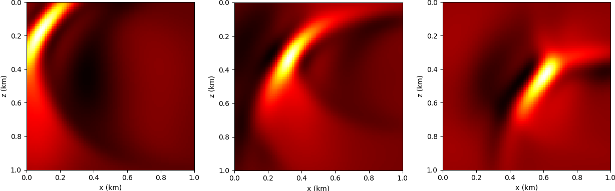
The second example aims to depict the qualitative character of objective landscape associated to the Lagrangian in eq. \(\eqref{eqlagrredscal}\). We setup a \(5\) km-by-\(10\) km velocity model linearly increasing with depth, \(v_{\beta}(x,z)=v_0+\beta\,z\), with \(v_0=2000\) m/s and \(\beta\) ranging from \(0.5\) to \(1\). A single source is located at \((x,z)=(0,0)\), and the data are recorded at the surface \(z=0\) with \(x\) varying from \(9\) km to \(10\) km.

We plot the values of the Lagrangian on the two-dimensional space discretized by the pairs \((\mathbf{m}_i,\mathbf{y}_j)\), where \(\mathbf{m}_i\) is the squared slowness associated to the velocity \(v_{\beta_j}\), and \(\mathbf{y}_j=\mathbf{d}-F(\mathbf{m}_j)\,\mathbf{f}\) is the data residual for \(\mathbf{m}_j\). The range of value of \(\beta\) has been chosen to produce severe cycle skipping, as it can be observed in the vertical slices (\(\mathbf{y}\) fixed) and diagonal slices of the objective landscape in Figure 3. Note that the diagonal slice represents qualitatively the classical FWI scenario, as it can be seen by substituting \(\mathbf{y}=\mathbf{r}\) in eq. \(\eqref{eqlagrredscal}\), under the assumptions \(\varepsilon\approx0\) and \(||\mathbf{r}||\approx c||F(\mathbf{m})^*\mathbf{r}||\), for an \(\mathbf{m}\)-independent constant \(c\). This shows the limitations of reduced space approaches. However, when the search space is augmented, the singular loci shown in Figure 3 can be circumvented.

BG compass inversion

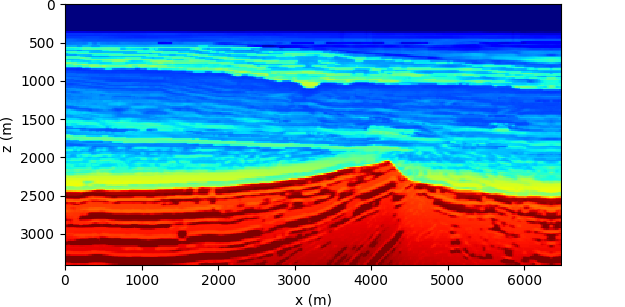
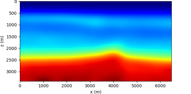
We show an inversion result obtained with the dual formulation object of this paper. The model here considered is the BG compass, shown in Figure 4a. The data consist of \(50\) shot gathers, and is collected by \(251\) receivers positioned at the surface. The time source function is a Ricker wavelet with a peak frequency of \(6\) Hz. The starting background model is depicted in Figure 4b.

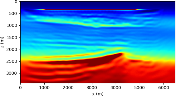
We ran \(10\) iterations of an alternating update optimization (each iteration consisting of one \(\mathbf{m}\) update and one \(\mathbf{y}\) update). For both experiments, the water layer is kept fixed throughout the inversion. We imposed the velocity values to be constrained on the interval \(1400\)–\(4700\) m/s. No other regularization scheme is used.

This example is notoriously challenging for conventional FWI, as it displays high/low velocity inversion near the water bottom. This generates poor updates with an inadequate starting guess. The results, depicted in Figure 4c, seem to indicate a relative robustness of the current method over these issues.

Summary

We introduced a dual formulation of full-waveform inversion: starting from the denoising problem, where we optimize the wave-equation fit with a data-misfit constraint, we offer a model extension by means of Lagrangian multipliers which belong to the data residual (dual) space and can be conveniently stored during the optimization. As in WRI, the formulation entails the solution of an augmented wave equation, where the physical source is complemented by an additional one governed by the multiplier. The augmented system is determined, and therefore can be solved in time domain with traditional time-marching solvers, along with the evaluation of the Lagrangian and its gradient computation. Moreover, we do not need to resort to continuation strategies to adapt weighting parameters in the augmented wave equation. We introduced an automatic scaling procedure to resolve the ill-conditioning of the Lagrangian, which would result in an unbalanced contribution of the physical and backpropagated sources in the augmented wave equation. Due to robustness and computational feasibility, the method is an enticing prospect for large-scale seismic inverse problems.

Acknowledgments

The implementation of the method described in this paper leverages on the Devito framework, which allows the automatic generation of highly-optimized finite-difference C code, starting from a symbolic representation of the wave equation (Luporini et al., 2018; Louboutin et al., 2018). In Julia, we interface to Devito through the JUDI package (Witte et al., 2019).