Removing density effects in LS-RTM with a low-rank matched filter

Abstract

Least-squares reverse-time migration faces difficulties when it inverts the data containing strong components related to density variation with velocity-only Born modeling operator. The strong density perturbation will be inverted as strong dummy velocity perturbations, which influence the amplitudes and phase of the velocity perturbations in the inverted model. The traditional method is to invert the additional density variations by developing Born operator with respect to both density and velocity or modify the image condition. In this work, we develop a matched-filter based LS-RTM for velocity-only Born modeling operator, which removes the artifacts in the imaging created by the strong density variation. This method doesn’t call for extra work of finite difference stencil and is more general. In the experiment part, we use a complex discontinuous layered medium with strong density variations at the ocean bottom, and show the efficacy of the propose formulation.

Introduction

Least-squares reverse-time migration (LS-RTM, Guitton et al. (2006); Dai et al. (2012); R. E. Plessix et al. (2002)) tries to fit observed reflection data in a least-squares sense to overcome RTM’s shortcomings in producing high resolution and high-fidelity amplitudes. In other words, LS-RTM attempts to invert the linearized Born modeling operator iteratively whereas RTM directly treats the adjoint of that operator as its inverse. So far, LS-RTM has demonstrated an ability to produce high-resolution images in combination with an efficient computational framework (F. J. Herrmann et al., 2015; Yang et al., 2016), overcoming drawbacks of overfitting artifacts (Herrmann and Li, 2012) caused by minimizing the \(\ell_2\) norm.

In addition to the developments listed above, people working on LS-RTM made lots of progress on incorporating multi-parameters (elastic parameters (Duan et al., 2016), visco-acoustic parameters (Dutta and Schuster, 2014) and so on) for complex geological structures. The corresponding Born modeling operators are linearized with respect to these elastic parameters, which allow us to mimic the elastic wave-propagation effects during the inversion. While important progress has been made handling elastic effects— e.g. by grouping subsets of elastic parameters that give rise to different radiation patterns (Operto et al., 2013)— working with multiple elastic parameters remains challenging.

Among the different parameters that rule the leading order behaviour of wave propagation, we count velocity and density as the most important pair (Beylkin et al., 1987). The products of these two, i.e., the seismic impedance, determines the amplitudes of the seismic waves to leading order. Perturbations in density generate reflection events even for a constant velocity model. This means that if we invert data generated by strong density perturbations with a Born modeling that accounts for velocity changes only we can expect strong artifacts degrading the quality of migrated images (Przebindowska et al., 2012, R. Plessix et al. (2013)). There are two main reasons for these artifacts: (i) the wavefields scattered by the velocity and density parameters exhibit similar behaviours for some scattering angles (Operto et al., 2013), and (ii) if we only invert for velocity perturbations without incorporating the true density perturbations in Born modeling operator then LS-RTM will try to fit the amplitudes and phase of the observed seismic data in terms of velocities only (Bai et al., 2014). This can lead to dummy reflection events in the LS-RTM along with incorrect amplitudes and phase distortions of the true reflectivity yielded by the velocity perturbations.

In this work, we propose to use a matched-filter approach to remove artifacts caused by strong unmodeled density perturbations in the context of imaging with surface-related multiples. Specifically, we are interested in imaging based on linearized inversions that derive from velocity-only acoustic Born modeling that handles strong water-bottom multiples generated by strong density changes at the ocean bottom. We find that the proposed matched-filter, when organized as a matrix, exhibits low-rank structure. This is due to the fact that the matched-filter tries to approximate the difference between radiation patterns of velocity and a (strong ocean bottom) density contrast, which varies smoothly with offset. Inspired by this observation, we propose to simultaneously estimate velocity perturbations and a low-rank matched-filter, which maps nonlinear (observed) data that contains components related to both density and velocity perturbations into “linearized” data close to data generated by Born modeling for perturbations in velocity only. The proposed method does not require the explicit Born operator for density but does need terms that depend on a smoothly varying background density.

Our paper is organized as follows. First, we form the objective function for our extended LS-RTM with a low-rank matrix constraint on the matched filter and conclude by describing a computationally efficient algorithm. Next, we evaluate the performance of the proposed approach on a quasi-layered model with faults where the density varies strongly at the ocean bottom. Finally, we show the benefits of inverting for the matched filter to correctly image both the amplitude and phase of the reflectivity for imaging problems that contain a strong density contrast at the ocean bottom.

Methodology

We start with a brief overview of LS-RTM, and then propose a matched-filter based formulation to handle strong density-related effects in imaging. As we mentioned before, LS-RTM attempts to minimize the \(\ell_2\) norm of the data residual between the observed and synthetic data by solving the following (unconstrained) optimization problem: \[ \begin{equation} \begin{aligned} \min_{\vector{x}} f(\vector{x}) = \sum_{i=1}^{n_f} \ & \Vert \vector{B}_i - \ctensor{J}_i(\vector{m}_0)(\vector{x}) \Vert_{F} , \end{aligned} \label{OBJ} \end{equation} \] where \(\ctensor{J}_i(\vector{m}_0)\) represents the monochromatic Jacobian with respect to velocity for all shots and followed by a matrication putting monochromatic shots in its columns. The vector \(\vector{x}\) stands for the unknown velocity perturbations. Finally, the matrix \(\vector{B}_i\) is the \(i^{th}\) frequency slice of the observed (nonlinear) data in the S-R domain (source-receiver domain). In this work, we think of non-linear data as the difference between the response of the “true earth”—i.e., a “hard” model for velocities and densities and the response of a “smoothed background earth” where both velocity and density vary smoothly. The symbol \(\Vert \cdot \Vert_F\) denotes the Frobenius norm. The above equation entails a “velocity only” linearization, which is accurate in the absence of strong density variations and a good background velocity model with respect to which the linearization is carried out. Under those conditions, equation \(\ref{OBJ}\) can produce good quality migrated images, which can then be used to perform reservoir characterization.

However, if the observed seismic data contains strong density effects generated by a strong ocean bottom, then the linearization undergirding equation \(\ref{OBJ}\) is no longer valid and as a consequence this may lead to a degradation in quality of migrated images (Przebindowska et al., 2012, R. Plessix et al. (2013)). One way to address this issue is to include density into equation \(\ref{OBJ}\) and re-linearize the Born modeling operator with respect to both velocity and density. While this approach is certainly a viable option, it is challenging and perhaps excessive to form a Born modeling operator that includes density, especially because it is well known that simultaneously inverting for both velocity and density is difficult because the two parameters have similar radiation patterns for certain scattering angles (Operto et al., 2013). As a result, LS-RTM runs the risk to map the perturbations in density to the velocity, which results in crosstalk in the imaging (Bai et al., 2014).

To address these issues, we propose to include a matched filter, which allows us to compensate for certain leading order density effects while inverting for the velocity perturbations only. Under the assumption that we can find such a matched filter \(\vector{M}\), we modify equation \(\ref{OBJ}\) as follows: \[ \begin{equation*} \min_{\vector{x},\vector{M}_i} f(\vector{x},\vector{M}_i) = \sum_{i=1}^{n_f} \Vert \vector{B}_i \vector{M}_i - \ctensor{J}_i(\vector{m}_0)\vector{x} \Vert_{F} , \end{equation*} \] where \(\vector{M}_i\) is the matched filter matrix for \(i^{th}\) frequency. As in our earlier work involving on-the-fly source estimation (Tu et al., 2013,Yang et al. (2016)), we use variable projections to solve for \(\vector{M}_i\) while minimizing the above objective with respect to the velocity perturbations collected in the vector \(\vector{x}\). However, contrary to finding a single time signature for the wavelet, the above matched filter involves for each frequency a full wavefield opening the risk of overfitting. To counter this problem, we control the rank \(k_i\) for each frequency. We motivate this choice by the fact that the difference in radiation patterns of velocity and the strong density contrasts at the ocean bottom vary smoothly over offset and we use this to stabilize the inversion. We now solve \[ \begin{equation} \begin{aligned} \min_{\vector{x},\vector{M}_i} f(\vector{x},\vector{M}_i) = \sum_{i=1}^{n_f} \ & \Vert \vector{B}_i \vector{M}_i - \ctensor{J}_i(\vector{m}_0)\vector{x} \Vert_{F} ,\\ & \text{s.t.} \ \text{rank}({\vector{M}_i})=k_i, \end{aligned} \label{OBJ1} \end{equation} \] For simplicity, we will now focus on solving the above problem for one single frequency and drop the subscript \(i\) accordingly and implicitly sum over frequencies, i.e., \(\sum_{i=1}^{n_f}\) for the remainder of this section. As we mentioned before, we solve the above problem \(\ref{OBJ1}\) with variable projections (Golub and Pereyra, 2003, Tu et al. (2016), Yang et al. (2016)). This involves computing gradient steps with respect to \(\vector{x}\) that minimize the \(\Vert \cdot \Vert_F\) norm —i.e,

\[ \begin{equation} \vector{x}_{k+1} = \vector{x}_k + \mathbf{s} \nabla_{\vector{x}} f(\vector{x},\vector{M})|_{\vector{x}=\vector{x}_k, \vector{M}=\vector{M}_k}, \label{xupdate} \end{equation} \]

where \({s}\) is the stepsize. As prescribed by variable projection, we solve for \(\vector{M}\) by minimizing \(\ref{OBJ1}\) for \(\vector{x}_k\) fixed. Since rank-minimization problems are NP hard, we use its convex relaxation instead, i.e., we replace the rank constraint by a nuclear-norm constraint (B. Recht et al., 2010), following the strategy proposed by A. Y. Aravkin et al. (2014).

Numerical Experiments

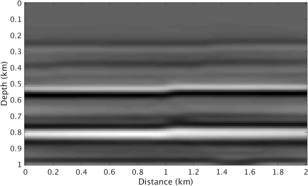
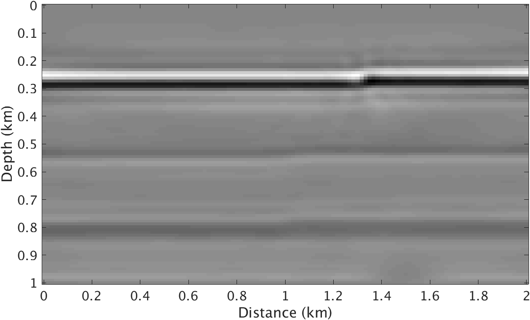
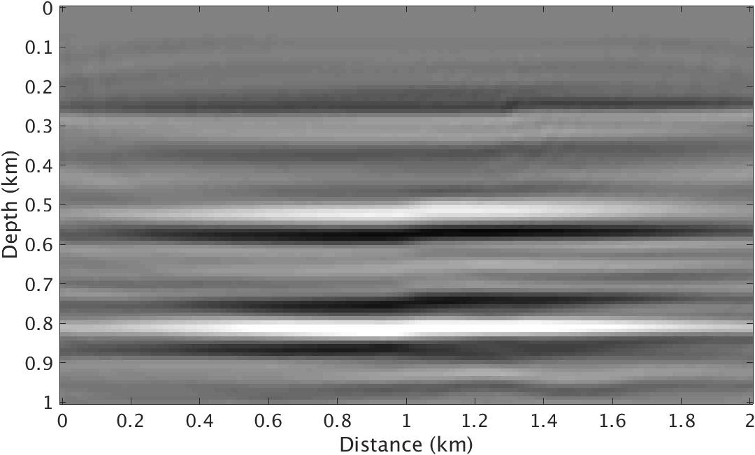
To test the performance of the proposed method, we conduct experiments on a quasi layered model with strong density contrast at the ocean bottom (Figure 1). Both velocity and density models are \(1\mathrm{km}\) deep and \(2\mathrm{km}\) wide and the underlying grid is discretized to \(10\mathrm{m}\). The background velocity model \(\vector{m}_0\) and background density model \(\vector{\rho}_0\) are smooth version of the true velocity and density models respectively and kinematically correct. We use a Ricker wavelet centered at \(10\mathrm{hz}\) as source wavelet and record the data for 4 seconds. The \(100\) shots and \(100\) receivers are spread over the model with \(10\mathrm{m}\) spacing. To test this method on this model, we compare the image inverted from ideal linearized data related to velocity perturbation and images inverted from nonlinear data with and without the matched-filter approach.

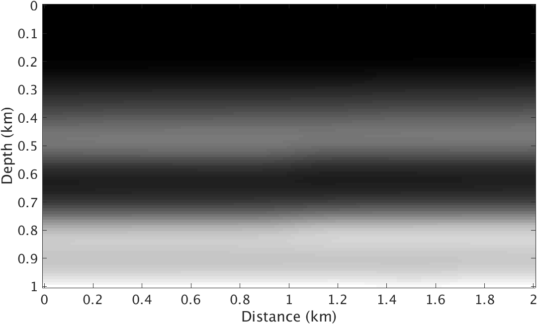
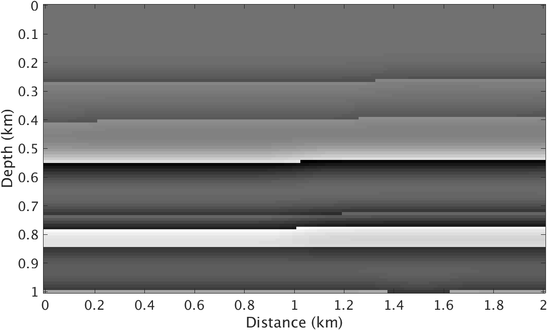
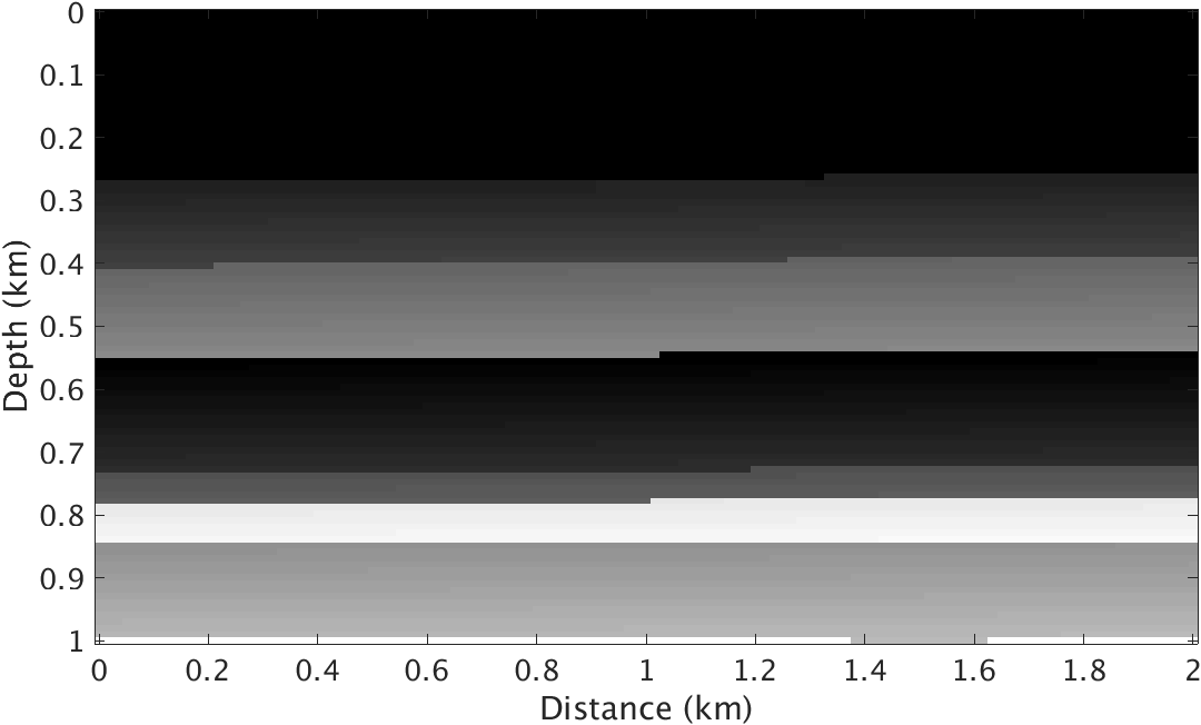
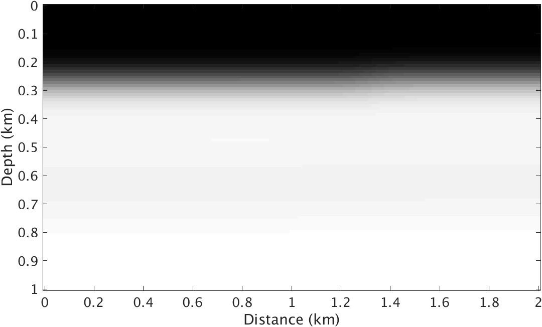
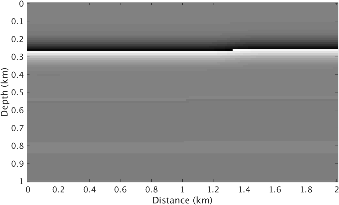
Given the true velocity and density models and their backgrounds, we generate “observed” nonlinear data by subtracting the response of the background models for varying velocity and density from the response yielded by the true velocity and density models. We compare this response with linear data obtained by applying linearized velocity only Born scattering operator to the true velocity perturbations plotted in Figure 1.

The monochromatic frequency slices of the linear data, nonlinear data and the matched-filter matrix \(\vector{M}\) at 5 and 10 Hz are shown in Figure 2. It is clear from the figures that the estimated matched-filter varies smoothly across sources, thus, exhibits low-rank structure. These results also validate our belief that the the difference between radiation patterns of velocity and the strong density contrast exhibits smooth structure over offset.

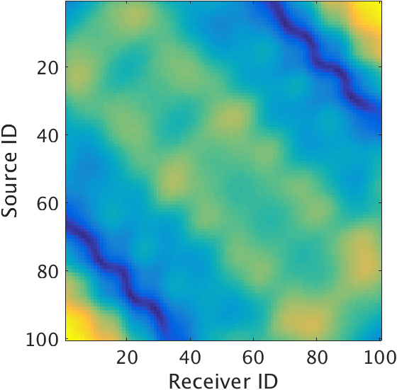
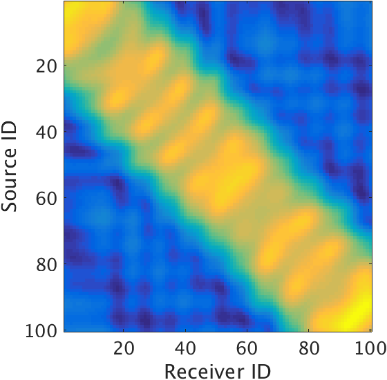
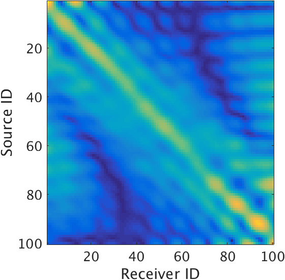
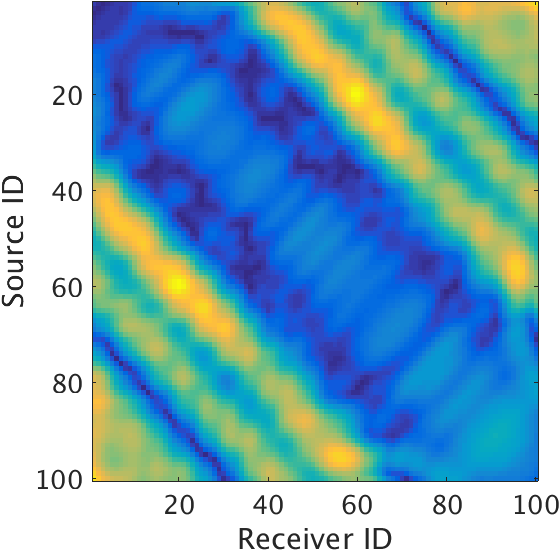
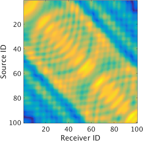
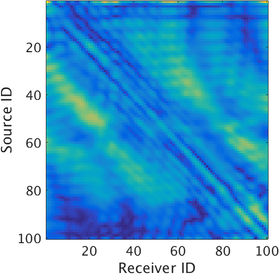
Figure 3a shows the idealized LS-RTM results using the linearized data (Figure 2a). We can see that for the ideal scenario, the layer interfaces are sharp and amplitudes are in the correct range. Also it is clear that the velocity perturbations at shallower interfaces especially at the ocean bottom are much weaker than those at the deeper interfaces. Next, we invert the non-linearized data (Figure 2b) without any matched-filter approach using the velocity-only Born modeling operator. It is evident from the inverted image (Figure 3b) that the LS-RTM maps the strong density perturbations to the velocity perturbations, thus, creating the dummy strong reflectors at the ocean bottom. Moreover, the amplitudes and phase of the subsequent deeper reflectors are wrong. Finally, we use the proposed matched-filter approach to perform the LS-RTM (Figure 3c). Using the propose method, we are able to remove the effects of the strong density perturbations at both the shallow and deeper sections. Thus, the estimated matched-filter can handle the strong density perturbation related effects while inverting for the velocity perturbation only, and can successfully remove the crosstalk created by density perturbations.

Conclusions

In this abstract, we propose a matched-filter based least-squares reverse time migration formulation to remove the strong density variation related components in the observed data. In contrast to other methods which invert density as one additional output or reform image condition, our method doesn’t require the work related to finite difference. Our modified formulation invert for the matched-filter and velocity perturbation simultaneously that matching the nonlinear observed data to the linear data with respect to velocity-only. In the experiment part, we used a complex discontinuous layered model with strong density variations at ocean bottom to test our method. We showed that the proposed matched-filter approach can remove the artifacts from density perturbation and get artifacts free migrated image related to the velocity perturbation. Future work is to incorporate the surface related multiples into the formulation since strong density variation can leads to strong surface related multiples, which can further enhance the resolution of the inverted images.

Acknowledgements

This work was in part sponsored by the SINBAD project.