A debiasing approach to microseismic

Introduction

To make unconventional reservoirs economical for the production of oil & gas, hydraulic fracturing is a common practice adapted by the oil & gas industry. During hydraulic fracturing fractures are created, which give rise to microseismic events. To make drilling decisions and to prevent hazardous situations, we need accurate information on the location and temporal evolution of these fractures. Because microseismic waves carry important information about fracture’s location and origin time, the microseismic data recorded at surface or along a monitor well is often used to locate these fractures (Shawn Maxwell, 2014).

Because of the operational ease and option to cover wide aperture, surface receivers are widely used (Duncan and Eisner, 2010; Lakings et al., 2006). But the microseismic data recorded along the surface comes at a cost of poor signal to noise ratio (S/R) in comparison to the data recorded along a monitor well. This is because we record more ambient noise (Forghani‐Arani et al., 2012). Moreover, microseismic waves suffer from attenuation while travelling large distance from subsurface to the surface receivers (S.C. Maxwell et al., 2013), which makes them difficult to observe in noisy data. Thus, low S/R of surface microseismic data poses a big challenge in terms of estimation of accurate location and the origin time of microseismic sources. For example, travel-time picking based methods rely on accurate picking of first arrivals of P and S-phases. When the noise levels are high, it becomes difficult to accurately pick these first arrivals (Bolton and Masters, 2001). Sometimes, the weak signal is not even visible to be picked.

In Sharan et al. (2016) & Sharan et al. (2017), we proposed a computationally efficient sparsity promotion based method to invert for the microseismic source wavefield from which we extract locations and source-time functions of closely spaced microseismic sources. Our method works with noisy data with S/R as low as \(-1\) dB, but performs poorly as the S/R decreases further. Moreover, while our sparsity-promotion based method is able to give us a good estimate of the shape of the source-time function, its amplitude is often incorrect. To overcome these limitations, we propose a debiasing approach to handle the noise and correctly estimate the amplitude of the source-time function. Our proposed approach consists of two main steps. The first step involves curvelet based denoising along with sparsity promotion based microseismic source inversion to detect the location of the microseismic sources. Since noise and signal has different morphological behaviour in curvelet domain (Candes and Donoho, 2000) it is easy to separate the noise in curvelet domain (F. J. Herrmann and Hennenfent, 2008; Neelamani et al., 2008; Kumar et al., 2017). In the second step, we use the estimated source location and perform a wave-equation based debiasing step to get the source-time function with correct amplitudes.

This paper is organized as follows. We first discuss the challenges in terms of detecting the location and estimating the source-time function of microseismic sources in the presence of strong incoherent noise in the observed data. Next, we explain the basics of curvelet transform and the steps we are using to denoise the noisy observed data. Subsequently, we explain the debiasing step to get the correct amplitude of the source-time function. Finally, we show the efficacy of the proposed approach on a noisy dataset generated on a complex subset of the Marmousi model (Brougois et al., 1990).

Methodology

Fracturing of rocks during fracking causes emission of microseismic waves. The microseismic events causing this emission are mostly localized along the fracture tips. Therefore, we assume these microseismic sources to be sparse in space. In Sharan et al. (2016), we exploited the fact that microseismic sources are sparse in space and have finite energy along time to solve \[ \begin{equation} \min_{\vector{Q}} \quad \|\vector{Q}\|_{2,1} \quad \text{s.t.}\quad\|\mathcal{F}[\vector{m}] (\vector{Q}) - \vector{d}\|_2 \leq \epsilon, \label{eqBPDN} \end{equation} \] where \(\vector{Q} \in \R^{n_x \times n_t}\), with \(n_x\) being the size of spatial grid and \(n_t\) being the number of time samples, is a matrix representing the complete microseismic source field containing the spatial temporal distribution of different microseismic sources —i.e. the \((i,j)\) entry in \(\vector{Q}_{i,j} = {q}(x_i,t_j)\). \(\mathcal{F}[\vector{m}]=\vector{P}{\mathcal{A}[\vector{m}]}^{-1}\) is the linear operator modeling the \(2\)D time-domain acoustic wave-equation. The linear operator \(\vector{P}\) restricts the wavefield to the receivers. \(\mathcal{A}[\vector{m}]\) is the \(2\)D finite-difference time stepping operator parametrized by the squared slowness \(\vector{m}\) of the medium. The minimizaton problem \(\ref{eqBPDN}\) aims to find such a \(\vector{Q}\), which has a minimum \(\ell_1\)-norm in space and has a minimum \(\ell_2\)-norm in time while fitting the observed data \(\vector{d}\) within the noise level \(\epsilon\). As mentioned earlier, sparseness of microseismic source wavefield \(\vector{Q}\) in space justifies the choice of \(\ell_1\)-norm in space and finite energy of these microseismic sources justifies the choice of \(\ell_{2}\)-norm in time in Equation \(\ref{eqBPDN}\).

Problem \(\ref{eqBPDN}\) has a form very similar to the classic Basis Pursuit Denoising (BPDN) problem (Chen et al., 1998; Berg and Friedlander, 2008). In Sharan et al. (2016), we proposed a new algorithm tailored to solve a slightly modified version of the problem \(\ref{eqBPDN}\) for the situations when the forward modeling operator is ill conditioned and computationally expensive. We will discuss about this new algorithm in the next section.

Linearized Bregman algorithm

Motivated by the recent successful application of linearized Bregman algorithm (Yin et al., 2008; Lorenz et al., 2014) to solve sparsity promoting least-squares migration problem (Herrmann et al., 2015), in Sharan et al. (2016), we proposed to solve \[ \begin{equation} \min_{\vector{Q}} \quad \|\vector{Q}\|_{2,1} + \frac{1}{{2}{\mu}}\|\vector{Q}\|_F^2 \quad \text{s.t.}\quad \|\vector{\mathcal{F}}[\vector{m}] (\vector{Q}) - \vector{d}\|_2 \leq \epsilon, \label{eqSrcest} \end{equation} \] which is strongly convex and a relaxed form of the original classic BPDN problem \(\ref{eqBPDN}\). \(\|.\|_F\) is the Frobenius norm and \(\mu\) acts as a trade-off parameter between sparsity given by \(\ell_{2,1}\)-norm term and the Frobenious norm term. When \(\mu \uparrow \infty\), then Equation \(\ref{eqSrcest}\) is equivalent to solving the original BPDN problem \(\ref{eqBPDN}\). Solving Equation \(\ref{eqSrcest}\) can be achieved through a simple algorithm with few tuning parameters (Sharan et al., 2016). We estimate the location of microseismic sources as outliers in the intensity plot calculated as \(\vector{I}(\vector{x})=\mathrm{vec}^{-1}\left(\sum_{t}\mid\vector{Q}(\vector{x},{t})\mid\right)\) from the inverted source field \(\vector{Q}\), where \(\mathrm{vec}^{-1}(\cdot)\) reshapes a vector into its original matrix form. The temporal variation of the inverted source field \(\vector{Q}\) at the estimated source locations give the source-time function of microseismic sources.

To avoid fitting noise in the data, every iteration of linearized Bregman algorithm involves projecting the data residual \(\vector{r}\) (i.e. difference between predicted and observed data) on the \(\ell_{2}\) ball of size \(\epsilon\) (Sharan et al., 2016) \[ \begin{equation} \Pi_\epsilon (\vector{r}) = \max \left\{{0,1-\frac{\epsilon}{\|\vector{r}\|}}\right\}\,\vector{r}. \label{project} \end{equation} \] Linearized Bregman algorithm performs well in locating microseismic sources and estimating their source-time function when the data has low to moderate levels of noise. But this is not always the case, microseismic data can be very noisy— i.e. \(\epsilon \gg \|\vector{r}\|\). Higher value of \(\epsilon\) implies that the projection of data residual in Equation \(\ref{project}\) will give a vector with all zeros. Therefore, linearized Bregman fails to update the source field \(\vector{Q}\) at every iteration. By using a smaller value of \(\epsilon\) instead of the actual noise level, projection in the Equation \(\ref{project}\) works and we can get source field \(\vector{Q}\) updated in every iteration of linearized Bregman algorithm. But using a smaller value of \(\epsilon\) instead of actual noise level in data means linearized Bregman algorithm will invert for such a source field \(\vector{Q}\) which will also fit the noise. Hence, the inverted source field will have many false sources as we observe this phenomenon in the numerical experiment section. To avoid the above mentioned situations with very noisy data, we propose to incorporate curvelet based denoising step prior to applying linearized Bregman algorithm to invert for the location followed by a wave-equation based debiasing approach to get the source-time function with correct amplitude.

Curvelet based denoising

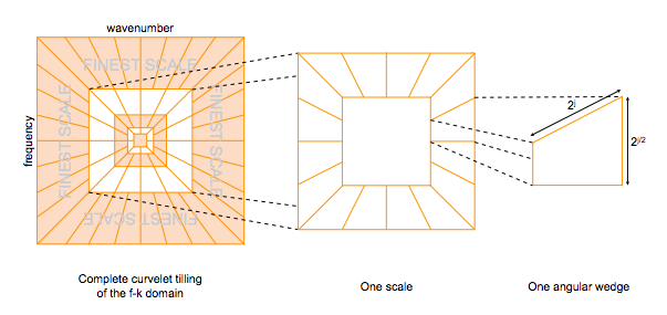
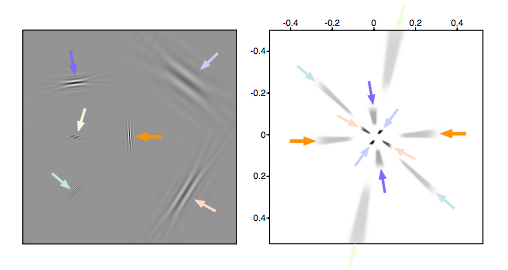
Microseismic signals recorded by the surface receivers are very weak in amplitude and are often contaminated with ambient noise that have similar or higher amplitude level than the amplitude of the microseismic signal present in the data (Forghani‐Arani et al., 2012). Also, the frequency range of the ambient noise is very similar to that of the microseismic signal (St-Onge and Eaton, 2011). This makes signal and noise separation very difficult and eventually causes problems in detecting the microseismic sources and estimating their source-time functions. Curvelet transform is a multi-scale and multi-directional transform (Candes and Donoho, 2000), that maps seismic data into angular wedges of different scales in the \(2\)D Fourier domain (Figure 1). This property of the curvelet transform helps in separating signals components based on their location, dip and scaling in the transform domain. Therefore, curvelet transform has been succefully used for incoherent (F. J. Herrmann and Hennenfent, 2008; Neelamani et al., 2008) and coherent noise attenuation (Kumar et al., 2017; Lin and Herrmann, 2013).

Motivated by prior successful application of curvelets, we propose following steps for denoising:

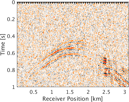
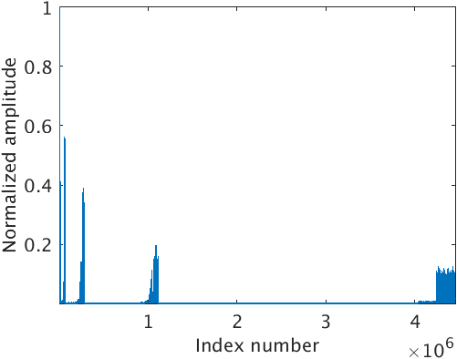
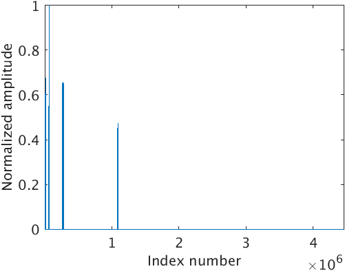
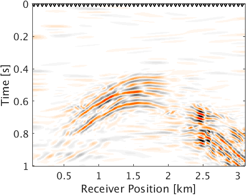
Line 2 in the Algorithm 1 corresponds to forward curvelet transform of the noisy microseismic data \(\vector{d}\) (Figure 2a) in the curvelet domain (Figure 2b). The indices in Figure 2b are arranged from coarse to fine scale. Line 3 corresponds to sorting of the absolute value of curvelet coefficients \(\vector{sb}\) in descending order. We also store the indices of the sorted curvelet coefficients in \(\vector{idx}\). Line 4 corresponds to computing the square root of normalized cumulative energy of the sorted curvelet coefficients. Line 5 corresponds to finding the smallest index \({p}\) in vector \(\vector{e}\) at which the square root of the normalized cumulative energy of sorted curvelet coefficient exceeds or is equal to the threshold \(\lambda\). In line 6, we form a subset \(\vector{R} \subseteq \vector{C}^\top\) of the inverse curvelet transform operator. Columns of \(\vector{R}\) correspond to the curvelet coefficients whose square root of the normalized cumulative energy in \(\vector{e}\) is greater than or equal to the threshold \(\lambda\). Line 7 corresponds to solving the normal equation to get the debiased and denoised curvelet coefficients \(\vector{b}_{dn}\) effectuated by the new inverse curvelet transform operator \(\vector{R}\). Debiasing neutralizes the shrinkage effect of thresholding and preserves energy. Figure 2c shows absolute value of the denoised and debiased curvelet coefficients \(\vector{b}_{dn}\) mapped to the corresponding location of the noisy curvelet coefficients \(\vector{b}\). Line 8 corresponds to taking inverse curvelet transform of the denoised curvelet coefficients \(\vector{b}_{dn}\) and taking its real part to get the denoised microseismic data (Figure 2d). We choose the threshold parameter as large as possible but for which we do not see any primary leakage in the difference plot.

The curvelet based denoising involves very few forward and inverse curvelet transform, which makes the proposed denoising method computationally cheap. To detect the location of microseismic sources from the denoised data \(\vector{d}_{dn}\) in a computationally efficient manner, we use the accelerated version of linearized Bregman algorithm (Sharan et al., 2017) along with a \(2\)D left preconditioner (F. J. Herrmann et al., 2009).

Debiasing of the source-time function

Given the location of microseismic sources, next step is to estimate the correct amplitude of source-time function. To achieve this, we use the forward modeling operator \(\vector{\mathcal{F}}[\vector{m}]\) and estimate source locations to fit the noisy data \(\vector{d}\) within some tolerance level. We use noisy data to avoid any kind of amplitude errors introduced in the approximated data by denoising. We now solve a debiasing problem using least squares as \[ \begin{equation} \tilde{\vector{W}} = \argmin_{\vector{W}\in\R^{n_t \times n}} \quad \|\mathcal{F}[\vector{m}](\vector{H}\vector{W}^\top) - \vector{d}\|, \label{eq:matee} \end{equation} \] where \(\vector{H}\in\R^{n_x \times n}\) is a matrix, with \({n}\) being the number of detected microseismic sources, whose \({i}^{th}\) column is \(\vector{h}_{i}\),which corresponds to the location of the \({i}^{th}\) source. \(\vector{h}_{i}\) is a spatial delta function \(\delta(\vector{x}-\vector{x}_{i})\) with \(\vector{x}_{i}\) being the location of \(i^{th}\) microseismic source. Equation \(\ref{eq:matee}\) solves for the unknown matrix \(\vector{W}\) whose \({i}^{th}\) column corresponds to the source-time function of \({i}^{th}\) microseismic source. We run only a few iterations of the unconstrained problem \(\ref{eq:matee}\) to avoid overfitting the noise in the data.

Numerical Experiments

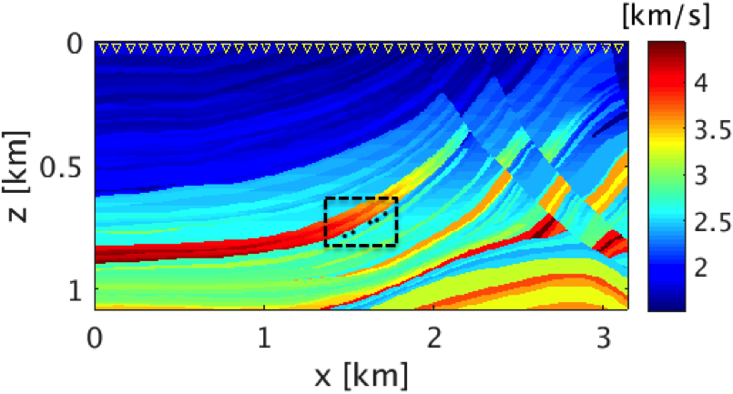
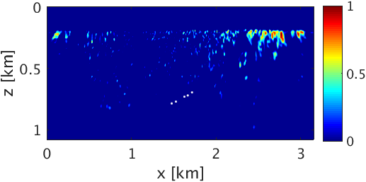
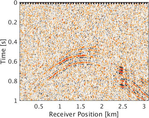
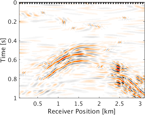
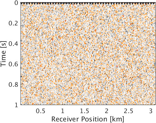
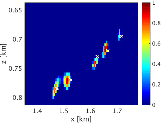
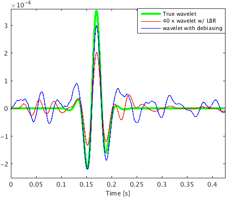
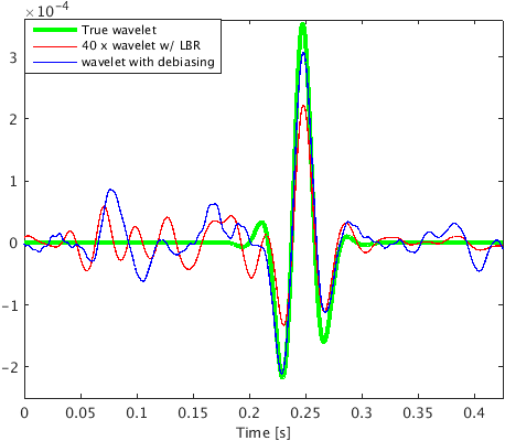
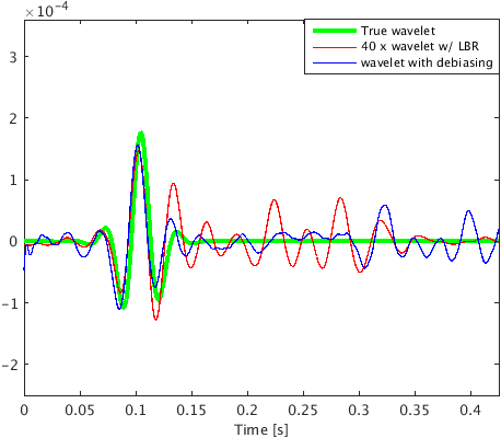
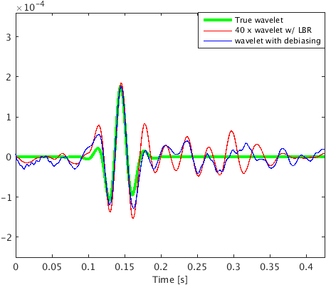
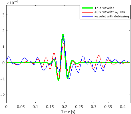
To demonstrate the effectiveness of our method for data with high noise level (S/R = \(-7.30\) dB), we performed a numerical experiment. We used \(2\)D acoustic finite-difference modeling code (Louboutin et al., 2017) to generate microseismic data of record length \(1.0\, \mathrm{s}\). To make the experimental setup more realistic, we used \(5\) microseismic sources of different amplitudes (differ by a factor of 2) and dominant frequencies \((30.0\,\), and \(25.0)\, \mathrm{Hz}\) activating at a small time interval with overlapping source-time functions to generate the microseismic data. Because of its geological complexity, we chose a part of Marmousi model with dimensions \(3.15\,\mathrm{km} \times 1.08\,\mathrm{km}\) (\(631 \times 217\) points) to perform the experiment. We place \(5\) microseismic sources (indicated by black dots in Figure 3a) in low velocity layer to generate the data. The adjacent sources are separated by half a dominant wavelength. We use surface receivers placed at a depth of \(20.0\, \mathrm{m}\) from the top surface to record the data. To get noisy data (Figure 4a) we add random noise (\(5.0\, \mathrm{Hz}\) to \(40.0\, \mathrm{Hz}\)) to the noise free data. We use kinematically correct smooth velocity model to invert for microseismic source field in the experiment. As expected, our method performs poorly without curvelet denoising and gives an intensity plot (Figure 3b) that is not very informative. This is because of the presence of lots of false sources in the estimated intensity plot (Figure 3b). Therefore, we apply the proposed curvelet based denoising steps to the noisy data (Figure 4a) to get denoised data (Figure 4b) with improved S/R of \(3.5\) dB. The difference plot (Figure 4c) between noisy (Figure 4a) and the denoised data (Figure 4b) shows that we do not loose any coherent signal with the proposed denoising method. With only \(10\) iterations of accelerated version of linearized Bregman algorithm, we are now able to locate all the \(5\) microseismic sources (Figure 4d) from this denoised data (Figure 4b). The white colour crosses in the estimated intensity plot correspond to the actual location of microseismic sources. All the outliers are located near the actual location of microseismic sources. To get the correct source-time function (blue colour plot in Figures 5a to 5e), we perform debiasing by least-squares using the estimated source location. We use the noisy data to perform this debiasing. Denoising helps us to get the correct source location and the debiasing step helps us to recover the source-time function with correct scaling. We further compare the source-time function (blue colour plot in Figures 5a to 5e) estimated by proposed approach to the source-time function estimated by Sharan et al. (2017) (red colour plot in Figures 5a to 5e). For visualization purpose, we scale the wavelets displayed in red color by a factor of \(40\). Thus, the proposed method can estimate the location and source-time function with correct scaling for microseismic data acquired in extremely noisy environment.

Conclusions

We proposed a debiasing based approach to estimate the location and source-time function of microseismic sources with correct amplitude from data with very low S/R. We showed ability of the proposed method to resolve microseismic events even when the sources are spatially close and have overlapping source-time functions. The proposed method is also computationally cheap as it requires very few forward and backward curvelet transforms along with few iterations of the accelerated version of linearized Bregman. Also, the source-time function estimation requires only a very few least-squares iterations. In future, we would like to apply PCA based denoising techniques to deal with different types of noise such as ground roll, source side noise etc.

Acknowledgement

This research was carried out as part of the SINBAD II project with the support of the member organizations of the SINBAD Consortium.