Effects of wrong adjoints for RTM in TTI media.

Mathias Louboutin¹*, Philipp Witte² and Felix J. Herrmann¹
1. Georgia Insitute of Technology, department of Computational Science and Engineering.
2. Seismic Laboratory for Imaging and Modelling (SLIM), University of British Columbia

Summary:

In order to obtain accurate images of the subsurface, anisotropic modeling and imaging is necessary. However, the twenty-one parameter complete wave-equation is too computationally expensive to be of use in this case. The transverse tilted isotropic wave-equation is then the next best feasible representation of the physics to use for imaging. The main complexity arising from transverse tilted isotropic imaging is to model the receiver wavefield (back propagation of the data or data residual) for the imaging condition. Unlike the isotropic or the full physics wave-equations, the transverse tilted isotropic wave-equation is not not self-adjoint. This difference means that time-reversal will not model the correct receiver wavefield and this can lead to incorrect subsurface images. In this work, we derive and implement the adjoint wave-equation to demonstrate the necessity of exact adjoint modeling for anisotropic modeling and compare our result with adjoint-free time-reversed imaging.

Introduction

Accurate representations of the physics are necessary for precise imaging of the earth’s subsurface. However, realistic representations of the physics are currently computationally infeasible, due to the large computational cost associated with solving elastic wave equations. The acoustic isotropic approximation of the wave equation is considerably cheaper to solve, but does not account for anisotropic propagation effects that can be observed in a variety of geological settings, such as thin sedimentary layers below the resolution of the predominant source wavelength. To account for kinematic effects of anisotropic media, a variety of acoustic anisotropic approximations of the wave equation exist. One of the most popular anisotropic wave equations is the tilted transverse isotropy (TTI) representation (Thomsen, 1986; Alkhalifah, 2000), which assumes symmetries of the anisotropy around a tilted axis. TTI wave equations are computationally cheaper than elastic wave equations, fairly straight-forward to implement and kinematically more realistic than the isotropic approximations. Modeling in TTI media is well studied (Fletcher et al., 2009; Xu and Zhou, 2014; L. Zhang et al., 2005; Zhan et al., 2013), but the literature usually only covers forward modeling, while reverse-time migration (RTM) (Baysal et al., 1983; Whitmore, 1983) also requires solving the corresponding adjoint wave equation. A common approach for imaging, is to assume that the TTI equations are self-adjoint, since the true underlying physical system is self-adjoint, and to use the forward modeling operator for back propagation, by flipping the time axis of the input shot records. However, even though derived from the true physics, TTI wave equations are in the general case not self-adjoint and require rigorous derivations of the correct (discrete) adjoint wave equations. In this work, we analyze the importance of using correct adjoints of the TTI wave equation for imaging and compare it to using the time-reversed forward modeling operator. The wave equations in this study are implemented with Devito (Lange et al., 2017; Louboutin et al., 2018), a finite-difference domain-specific language (DSL) in Python, that allows symbolic implementations of forward and adjoint wave equations, from which optimized C code is automatically generated during runtime. Furthermore, we use the Julia Devito Inversion (JUDI) framework (Witte et al., 2018) for parallelizing over the source locations. In the next section, we start with the definition of the TTI wave-equation, the derivation of its adjoint and comparisons of impulse responses from the time-reversed and true adjoint TTI wave equation. We then compare RTM results of a realistic 2D TTI model and highlight the importance of exact adjoint modeling.

Theory

Transverse-isotropic wave equations provide a kinematically accurate acoustic representation of the physics with a reduced number of parameters in comparison to the general elastic wave equation (five parameters instead of 21). We refer to Thomsen (1986), Alkhalifah (2000) and L. Zhang et al. (2005) for a detailed derivation and justification of the formulation and concentrate here on the derivation of the adjoint TTI wave-equation and the its relevance for imaging. In a TTI medium, the governing equations with the conventional physical parametrization (squared slowness \(m(\mathbf{x})\), Thomsen parameters \(\epsilon(\mathbf{x}), \delta(\mathbf{x})\) and tilt and azimuth \(\theta(\mathbf{x}), \phi(\mathbf{x})\)) are given by (Thomsen, 1986, Y. Zhang et al. (2011), Duveneck and Bakker (2011)): \[ \begin{equation} \begin{aligned} &m(x) \frac{d^2 p(\mathbf{x},t)}{dt^2} - (1+2\epsilon(\mathbf{x}))(G_{\bar{x}\bar{x}} +G_{\bar{y}\bar{y}} )p(\mathbf{x},t) \\ &- \sqrt{(1+2\delta(\mathbf{x}))}G_{\bar{z}\bar{z}} r(\mathbf{x},t) = q, \\ &m(x) \frac{d^2 r(\mathbf{x},t)}{dt^2} - \sqrt{(1+2\delta(\mathbf{x}))}(G_{\bar{x}\bar{x}} +G_{\bar{y}\bar{y}} ) p(\mathbf{x},t) \\ &- G_{\bar{z}\bar{z}} r(\mathbf{x},t) = q, \\ \end{aligned} \label{TTIfwd} \end{equation} \] where \(G_{\bar{z}\bar{z}}, G_{\bar{x}\bar{x}}, G_{\bar{y}\bar{y}}\) are the rotated second order differential operators that depend on the tilt, azimuth and the conventional (isotropic) spatial derivatives \(\frac{d}{dx}, \frac{d}{dy}\) and \(\frac{d}{dz}\). As discussed in Y. Zhang et al. (2011) and Duveneck and Bakker (2011), we consider the discrete finite-difference representations of the three differential operators \(G_{\bar{z}\bar{z}}, G_{\bar{x}\bar{x}}, G_{\bar{y}\bar{y}}\) to be self-adjoint to ensure numerical stability. For example, we can choose: \[ \begin{equation} \begin{aligned} G_{\bar{x}\bar{x}} &= D_{\bar{x}}^T D_{\bar{x}} \\ D_{\bar{x}} &= cos(\theta(\mathbf{x}))cos(\phi(\mathbf{x}))\frac{d}{dx} + cos(\theta(\mathbf{x}))sin(\phi(\mathbf{x}))\frac{d}{dy} - sin(\theta(\mathbf{x}))\frac{d}{dz}. \end{aligned} \label{rot} \end{equation} \] The rotated finite-difference operators contain the angles of the TTI symmetry axis, which are assumed to be spatially varying as described in equation \(\ref{rot}\). The squared slowness and Thomsen parameters are spatially varying as well, under the assumption that \(\epsilon > \delta\). With the TTI system of equations as defined above, we consider the standard zero-lag cross-correlation imaging condition for reverse-time migration for the case of couple equations: \[ \begin{equation} I = \sum_{t=1}^{n_t} ( \ddot{p} p_a + \ddot{r} r_a). \label{TTIgrad} \end{equation} \] In the above expression, \(p_a, r_a\) are the two components of the adjoint (TTI) wavefields and \(\ddot{p}, \ddot{r}\) are the second order time derivatives of the two forward wavefields. Note, that the gradient is computed as the sum of the separate correlation of the two components, not the correlation of the sum of the components. Furthermore, the adjoint wavefields \(p_a, r_a\) cannot be computed by forward propagating the time-reversed shot records, but require solving the actual adjoint TTI wave equations. Even though the spatially varying finite-difference operators \(G\) are self-adjoint by construction, the overall system itself is not self-adjoint, since the operators are multiplied with terms that contain the spatially varying Thomsen parameters. The correct adjoint system of equations corresponding to the TTI forward wave equations (equation \(\ref{TTIfwd}\)) is given by: \[ \begin{equation} \begin{aligned} &m(x) \frac{d^2 p_a(\mathbf{x},t)}{dt^2} - \\ &(G_{\bar{x}\bar{x}} +G_{\bar{y}\bar{y}})((1+2\epsilon(\mathbf{x}))p_a(\mathbf{x},t) + \sqrt{1+2\delta(\mathbf{x})} r_a(\mathbf{x},t)) = q_a, \\ &m(x) \frac{d^2 r_a(\mathbf{x},t)}{dt^2} - G_{\bar{z}\bar{z}}(\sqrt{1+2\delta(\mathbf{x})} p_a(\mathbf{x},t) + r_a(\mathbf{x},t)) = q_a, \\ \end{aligned} \label{TTIadj} \end{equation} \] where \(q_a\) is the adjoint source, which, for RTM, are the observed shot records. Compared to the forward TT wave equations, the adjoint system is fundamentally different. While the forward system consists of two coupled PDEs that are merely two rotated and weighted acoustic wave-equations, the corresponding adjoint system consists of two fully decoupled horizontal/vertical equations. To illustrate the differences of the true adjoint wave equations and the time-reversed equations, we compare the impulse response of the subsurface for both cases by back-propagating a time-reversed Ricker wavelet, injected at a single receiver location.

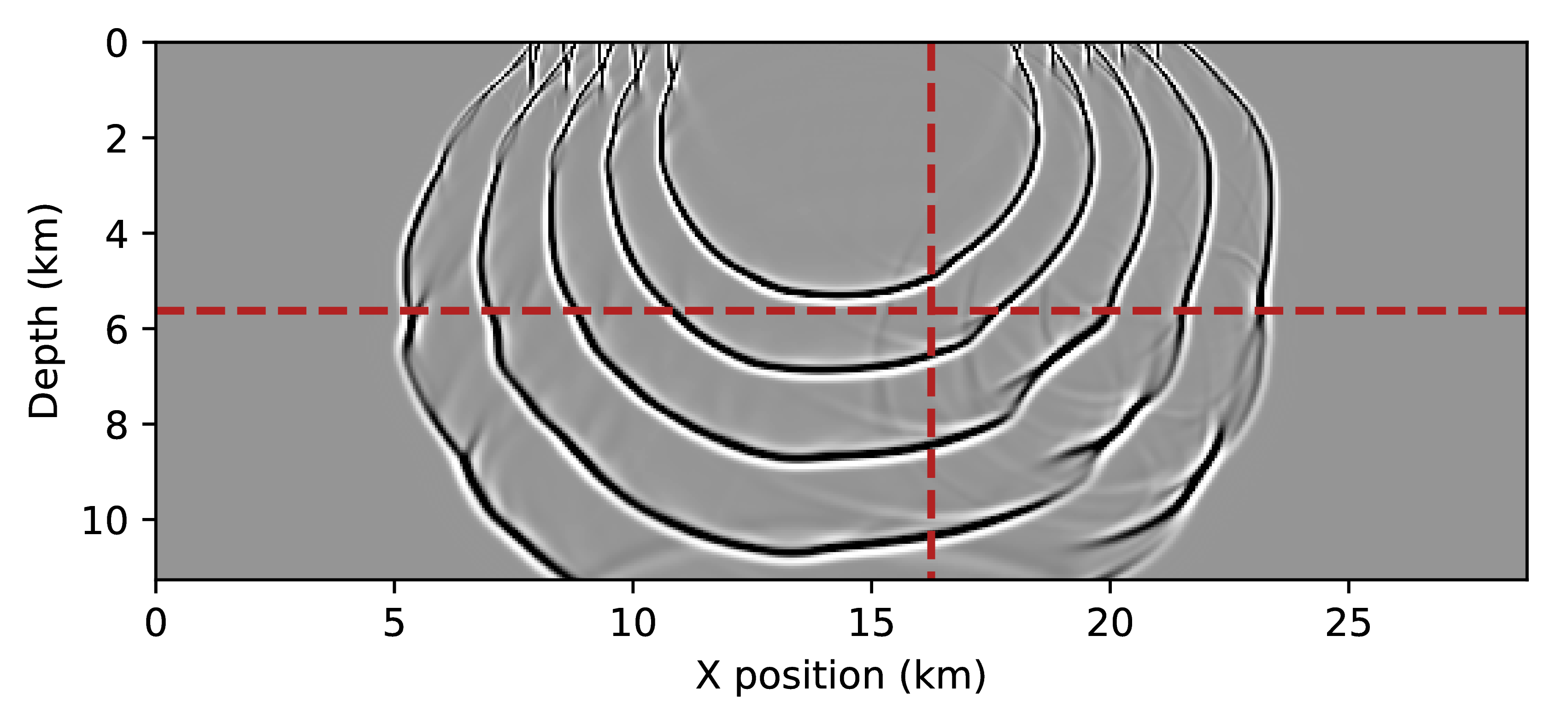
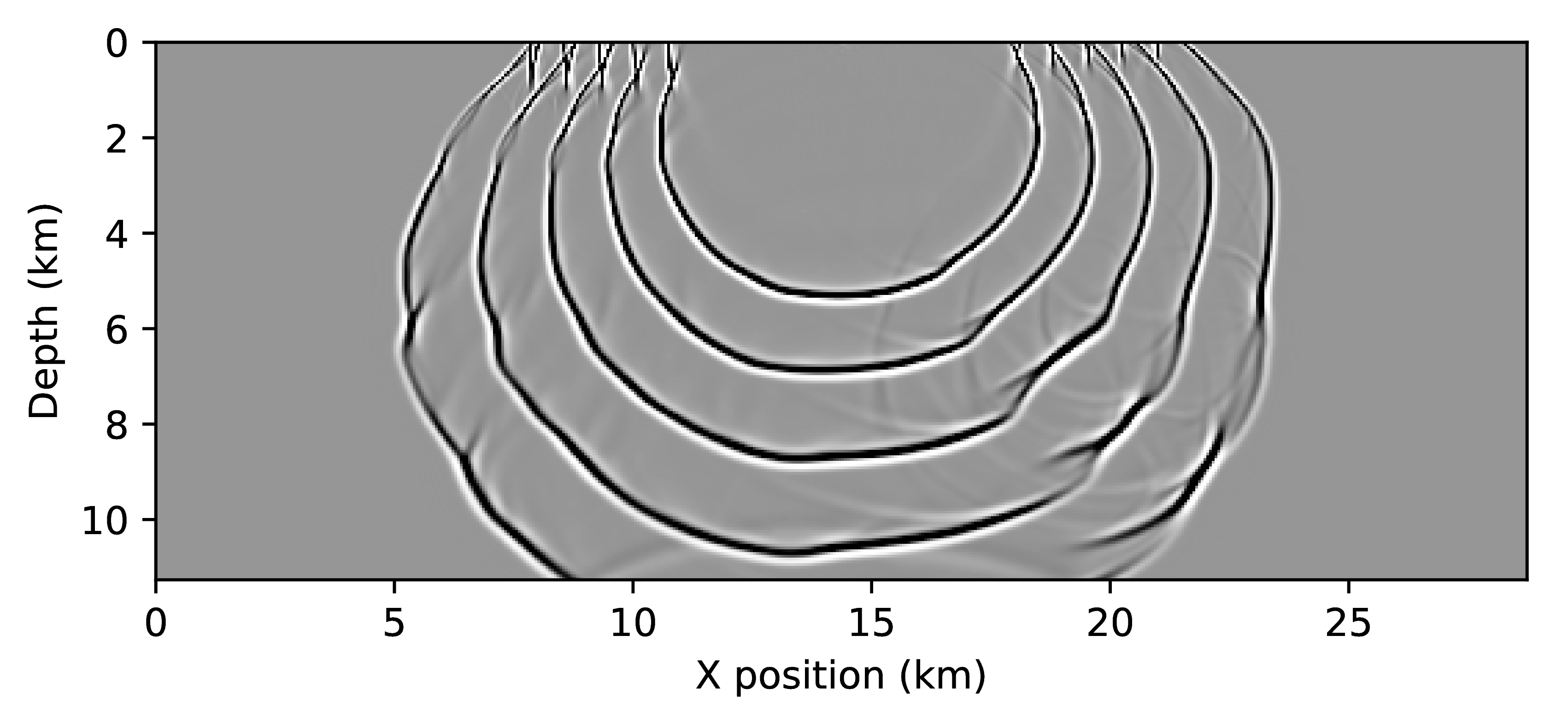
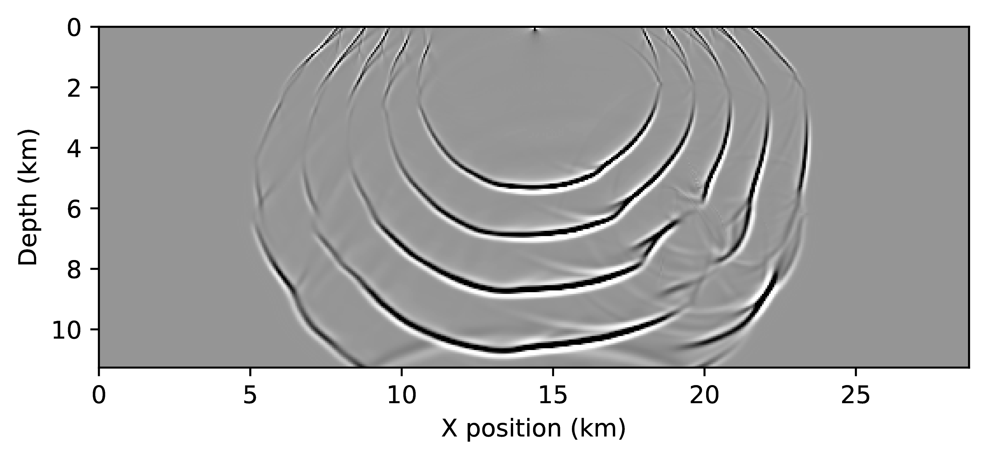
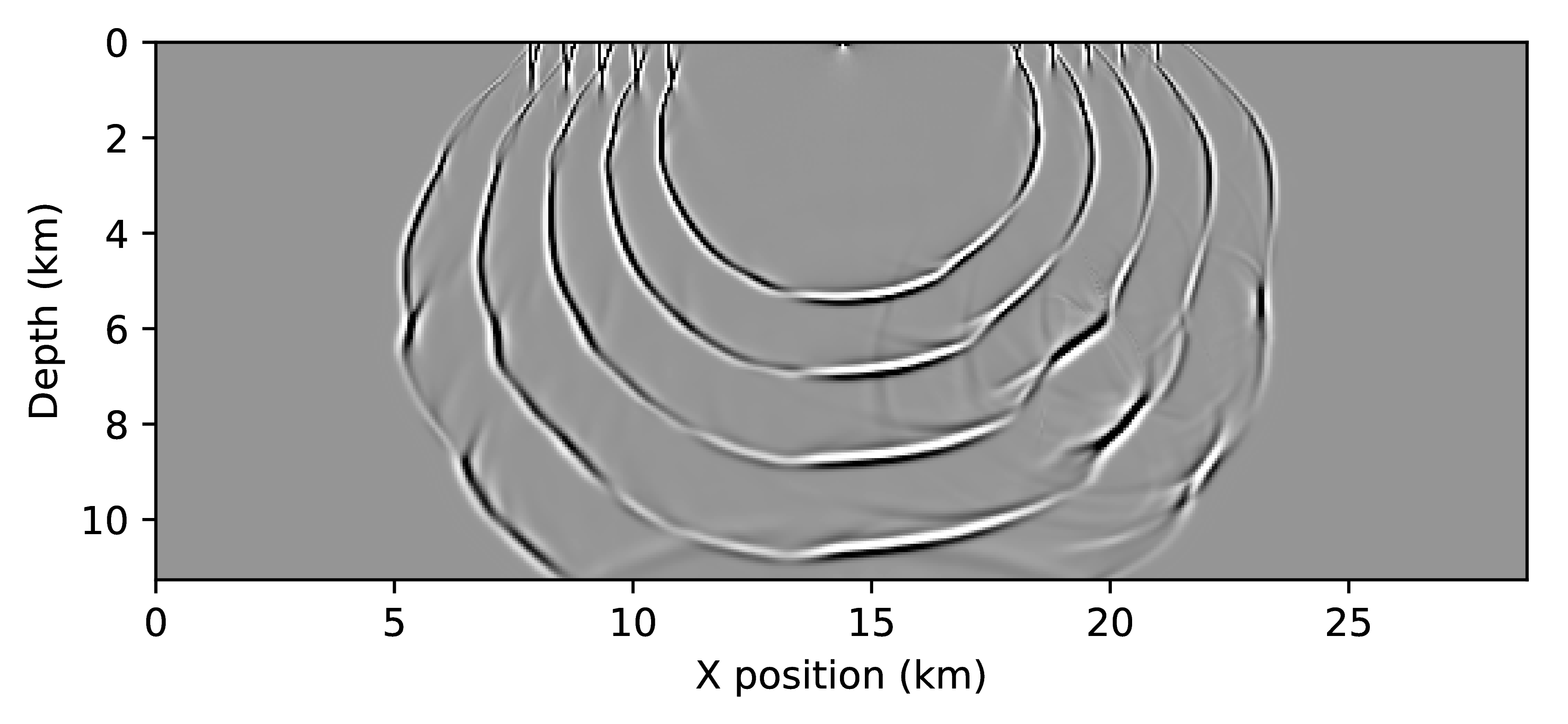
Figure 1 shows that the impulse responses of the time-reversed and adjoint TTI systems are drastically different. As expected, the amplitudes along the wave-fronts differ, since the adjoint wavefield consists of a purely vertical and a purely horizontal components, while the time-reversed wavefields are a combination of both. The difference plots in the bottom row of Figure 1 show that the amplitudes of wave fronts differ throughout the full domain and will therefore lead to different results, once correlated for an RTM image. Furthermore, we plot two traces of the wavefields that were extracted at the locations indicated by the red lines (Figure 2). While the amplitude difference in the snapshots may appear only minor, the trace plots reveal that the amplitude differences are in fact substantial. The vertical trace shows that the amplitude differs up to a factor of five and that the amount of energy in the two wavefield components seems to be flipped (i.e. \(p_a\) contains more energy than \(r_a\)). The most problematic differences can be observed in the horizontal trace comparison, where wee see that the energy of the wavefields is flipped between the left and right side of the wavefield (with respect to the source), which means the subsurface illumination of the time-reversed wavefield in incorrect.

Reverse Time Migration

We finally show a Reverse-Time-Migration (RTM) example on the 2007 BP TTI dataset. We compare in this example the images obtained with the true adjoint wavefields \(\eqref{TTIadj}\) and the time-reversed “adjoint” that propagates backward in time Equation \(\ref{TTIfwd}\) for the “adjoint” modeling. We use a 20 Hz Ricker wavelet and back propagate the muted data as in Sun et al. (2016) without any extra processing or filtering.

The two images do look similar, both contain the salt body and the anticline and complex events on the left. However there are a number of substantial differences between these two images that require a closer look. We show on Figure 4 three parts of the final image overlaid with the background velocity model. The three selected areas are highlighted in Figure 3 and are within the part of the model with a non zero tilt angle.

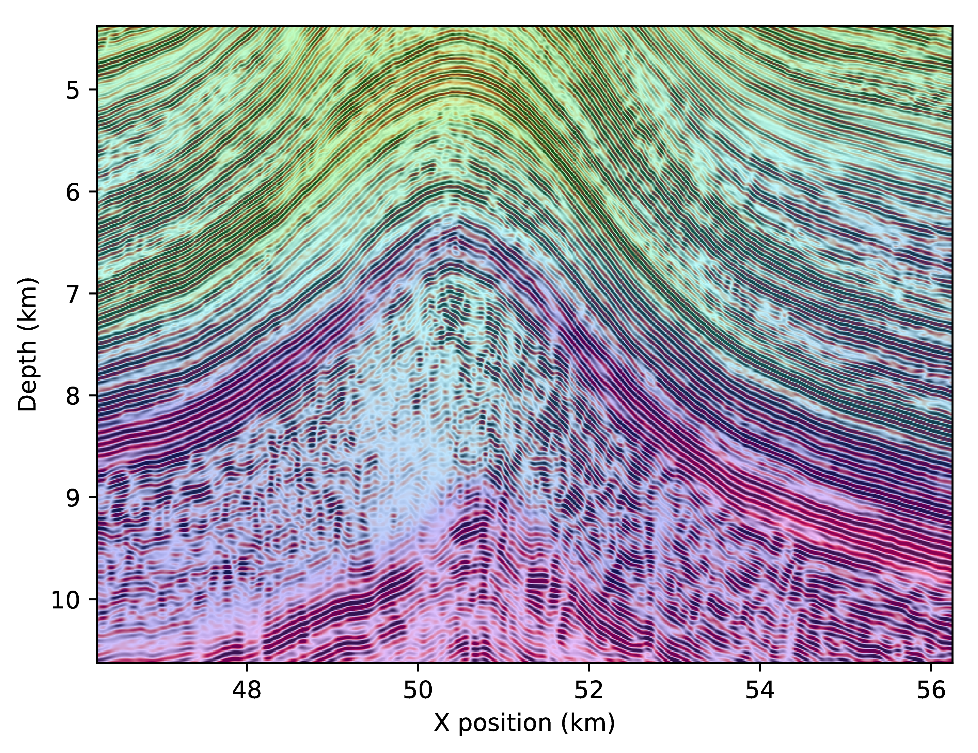
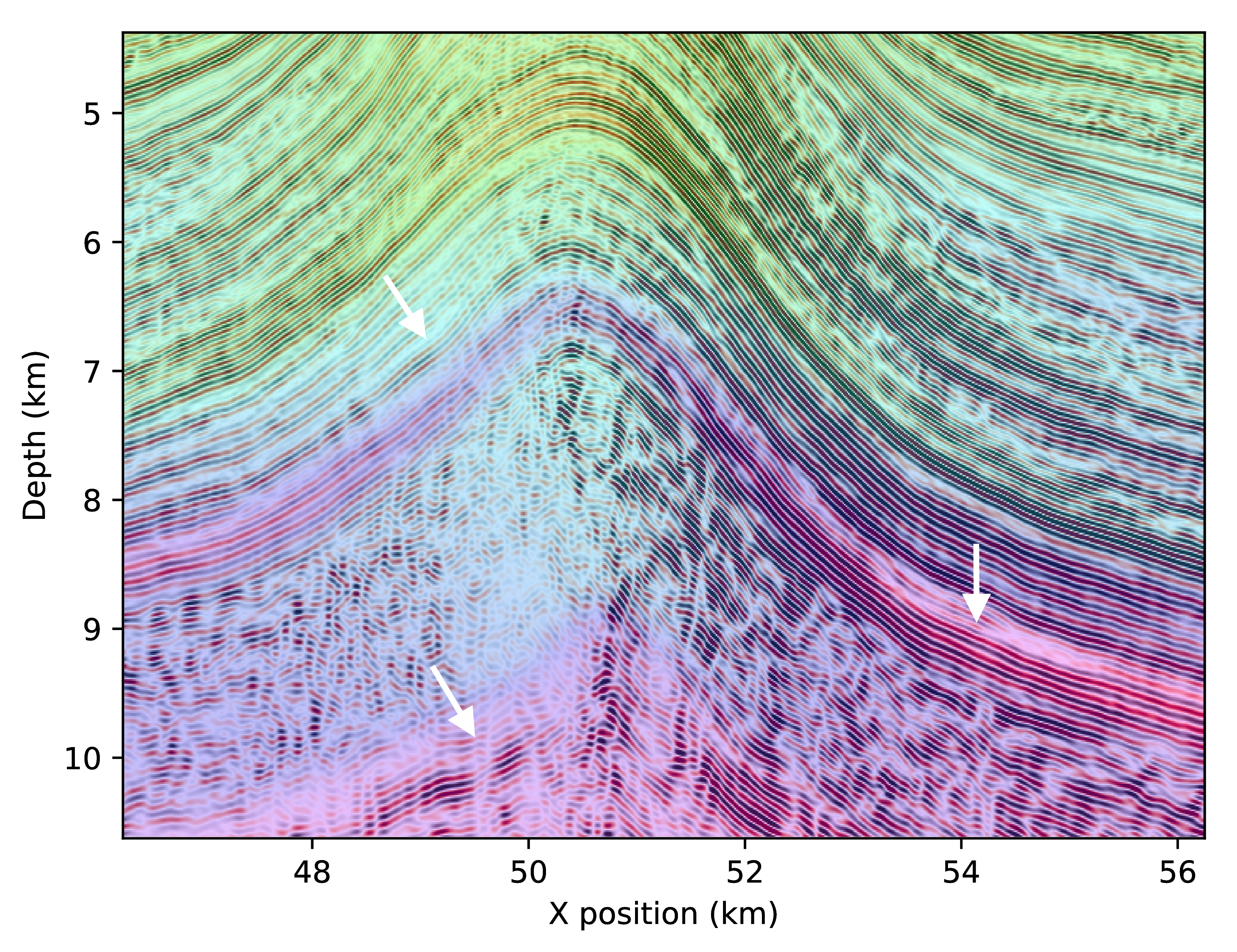
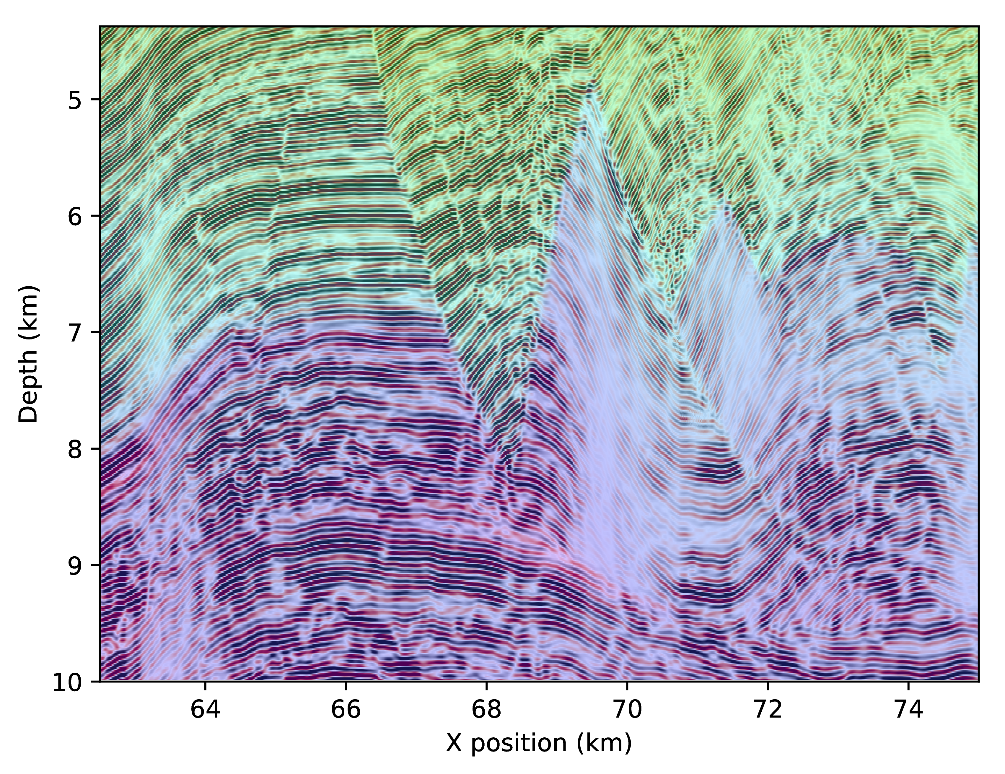
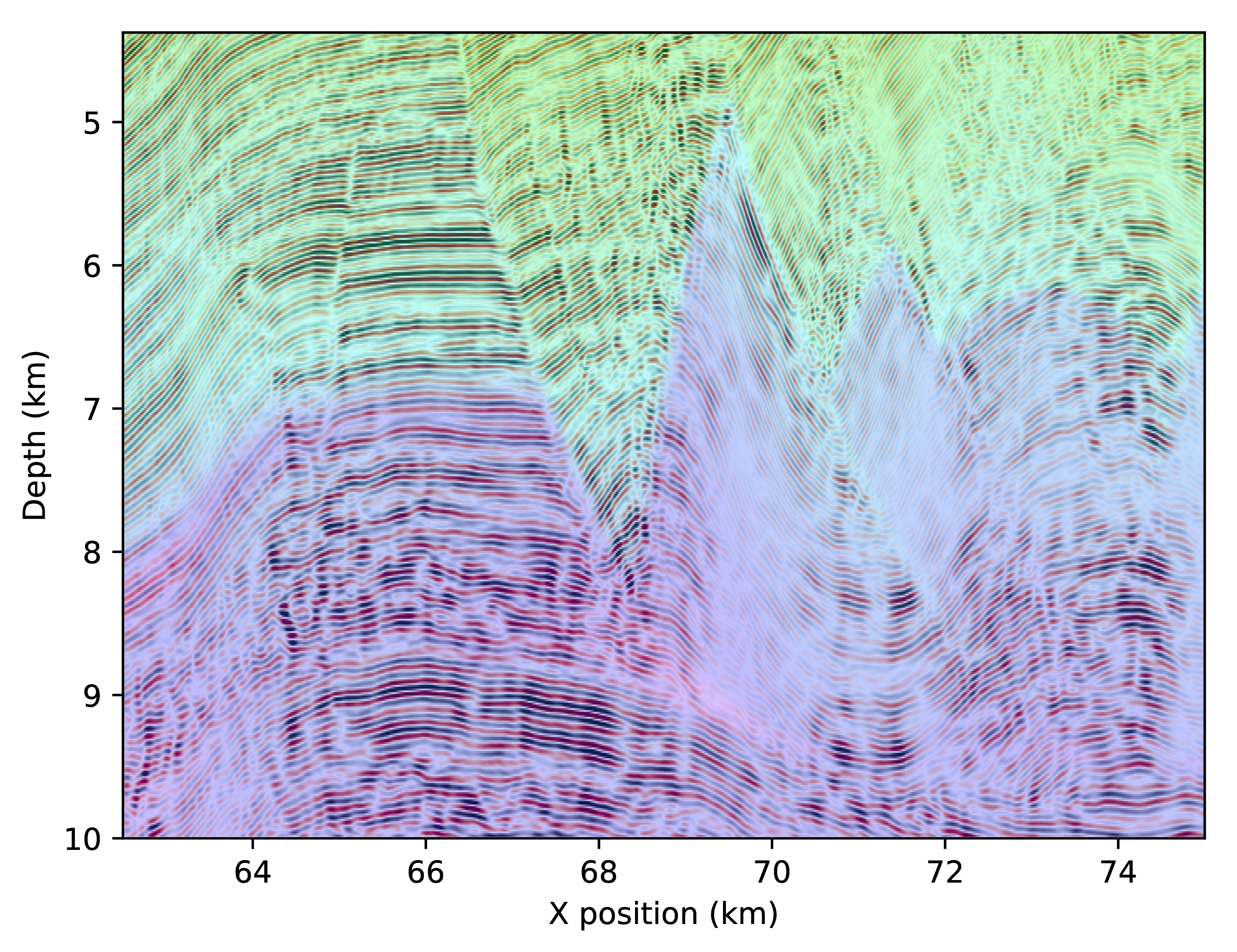
The first difference to notice on these zoomed images, is that the salt boundaries are imaged at incorrect positions with the adjoint-free time-reversed method. The bottom flat layer is too deep while the vertical channel is shifted to the left. On the second zoomed in part, we observe that the image obtained with the true adjoint is more focused and highlights more reflectors aligned with the velocity variations while the time-reversed one is missing a lot of reflectors on the left of the anticline. We also see that that the reflectors matching the high velocity at the bottom are blurry and too deep with the time-reversed method. Finally, on the last image, both methods focus at the correct positions, however, the time-reversed image is unfocused and has missing or blurred reflectors. While these differences may look minor, the shifts in space are in the order of hundred of meters and are non negligible errors for interpretation.

Conclusions

In this work, we detailed the main differences between adjoint-free time-reversal imaging and imaging with proper adjoints in a transverse tilted isotropic medium. We demonstrated on a realistic dataset that time-reversal does not image the subsurface correctly and that rigorous adjoint modeling is necessary for anisotropic imaging. Even though the time-reversed image perhaps seems good by itself, we showed that the subsurface events actually do not align with the velocity once overlaid. Such a displacement with good focusing could lead to incorrect interpretation. On the other hand, we demonstrated improved imaging accuracy with adjoint modeling that places subsurface events at the correct locations and creates a more focused image in several areas such as the anticline region.

Finally, adjoint modeling provides one extra tool that would not be possible with time-reverse imaging. While reverse-time migration does provide good images, complex model such as the one we presented here, requires a least-squares solution to image areas with poor illumination or steep events such as the flanks of the salt body. These least-square methods require an exact adjoint to stay stable and converge. With the correct adjoint implemented, the next step is to incorporate our simulator in a least-square imaging workflow to improve the final image.

Acknowledgements

This research was carried out within Georgia Institute of Technology, School of Computational Science and Engineering. This research was carried out as part of the SINBAD II project with the support of the member organizations of the SINBAD Consortium.

References

Alkhalifah, T., 2000, An acoustic wave equation for anisotropic media: Geophysics, 65, 1239–1250.
Baysal, E., Kosloff, D. D., and Sherwood, J. W. C. and, 1983, Reverse time migration: Geophysics, 48, 1514–1524.
Duveneck, E., and Bakker, P. M., 2011, Stable p-wave modeling for reverse-time migration in tilted tI media: GEOPHYSICS, 76, S65–S75. doi:10.1190/1.3533964
Fletcher, R. P., Du, X., and Fowler, P. J., 2009, Reverse time migration in tilted transversely isotropic (tTI) media: GEOPHYSICS, 74, WCA179–WCA187. doi:10.1190/1.3269902
Lange, Kukreja, Luporini, Louboutin, Yount, Hückelheim, and Gorman, 2017, Optimised finite difference computation from symbolic equations: In Katy Huff, David Lippa, Dillon Niederhut, & M. Pacer (Eds.), Proceedings of the 15th Python in Science Conference (pp. 89–96).
Louboutin, M., Witte, P. A., Lange, M., Kukreja, N., Luporini, F., Gorman, G., and Herrmann, F. J., 2018, Full-waveform inversion - part 2: Adjoint modeling: The Leading Edge, 37, 69–72. doi:10.1190/tle37010069.1
Sun, J., Fomel, S., and Ying, L., 2016, Low-rank one-step wave extrapolation for reverse time migration: GEOPHYSICS, 81, S39–S54. doi:10.1190/geo2015-0183.1
Thomsen, L., 1986, Weak elastic anisotropy: Geophysics, 51, 1964–1966.
Whitmore, N. D., 1983, Iterative depth migration by backward time propagation: 1983 SEG Annual Meeting, Expanded Abstracts.
Witte, P. A., Louboutin, M., Lange, M., Kukreja, N., Luporini, F., Gorman, G., and Herrmann, F. J., 2018, A large-scale framework for symbolic implementations of seismic inversion algorithms in julia:GEOPHYSICS.
Xu, S., and Zhou, H., 2014, Accurate simulations of pure quasi-P-waves in complex anisotropic media: Geophysics, 79, 341–348.
Zhan, G., Pestana, R. C., and Stoffa, P. L., 2013, An efficient hybrid pdeudospectral/finite-difference scheme for solving the TTI pure P-wave equation: Journal of Geophyics and Engineering, 10.
Zhang, L., Rector III, J. W., and Micheal, H. G., 2005, Finite-difference modelling of wave propagation in acoustic tilted TI media: Geophysical Prospecting, 53, 843–852.
Zhang, Y., Zhang, H., and Zhang, G., 2011, A stable TTI reverse time migration and its implementation: Geophysics, 76, WA3–WA11.