Massive 3D seismic data compression and inversion with hierarchical Tucker

Yiming Zhang*, Curt Da Silva, Rajiv Kumar, and Felix J. Herrmann
Seismic Laboratory for Imaging and Modeling (SLIM), University of British Columbia

Introduction

In recent years, industrial seismic exploration has moved towards acquiring data in challenging-to-image regions. In order to satisfy Nyquist sampling criteria and to provide more useful information in the deep or steeply dipping geologies, companies typically acquire finely-sampled and long-offset seismic data in order to avoid aliasing and inaccuracy in subsequent processing steps (Abma et al., 2007). Owing to the large scale and dimensionality of 3D seismic experiments, acquiring fully sampled data is an exceedingly time-consuming and cost-intensive process. For 3D seismic surveys, the high dimensionality (two source coordinates, two receiver coordinates and time) leads to exponentially increasing data processing costs as the size of the area of interest grows and fully sampled volumes can easily reach terabytes or even petabytes in size.

Terrain limitations or cost restrictions often limit fully sampling data in realistic scenarios. To mitigate the issue of missing traces or coarsely sampled data, so-called transformation-based methods typically try to transform the data into different domains, such as the Radon (Kabir and Verschuur, 1995; Wang et al., 2010), Fourier (M. Sacchi et al., 2009; Curry, 2010), Wavelet (Villasenor et al., 1996), and Curvelet (Hennenfent and Herrmann, 2006; Herrmann and Hennenfent, 2008) transforms, and exploit sparsity or correlations among coefficients in order to recover the fully sampled volumes. The authors in (Hennenfent and Herrmann, 2006; Herrmann and Hennenfent, 2008) successfully reconstruct incomplete seismic data in the Curvelet domain based upon the ideas from compressive sensing using \(\ell_1\)-based reconstruction. Although these methods are sufficient for storing and retrieving data due to the storage of small subsets of total coefficients, transform-based methods are unable to easily provide query-based access to elements of interest from the data volume such as common shot gathers. As such, if one recovers a subsampled volume with one of these techniques, invariably one must reform the entire data set before working with it in processes such as full-waveform inversion.

Alternate to transform-based methods are matrix completion (Oropeza and Sacchi, 2011; Kumar et al., 2015) and tensor completion (Kreimer and Sacchi, 2012; Trickett et al., 2013; Da Silva and Herrmann, 2015) techniques, which exploit the natural low-rank behavior of seismic data under various permutations. Critical in applying these methods to realistically-sized data is the absence of computing singular value decompositions (SVDs) on data volumes. Methods proposed by (Kreimer and Sacchi, 2012), for instance, which employ a projection on to convex sets technique to complete seismic data in the Tucker tensor format, suffer from the high computational complexity of such operations. As a result, practitioners often have to resort to working with small subsets or windows of the data, which may degrade the recovered signal (Kumar et al., 2015). An more computationally feasible approach is to formulate algorithms directly in terms of the low-rank components of the signal, which eliminates the necessity of computing expensive SVDs or resorting to aggressive data windowing. The authors in Da Silva and Herrmann (2015) develop an optimization framework for interpolating Hierarchical Tucker (HT) tensors using the smooth manifold structure of the format, which we explore further.

In this work, we outline a workflow for interpolating seismic data from missing traces directly in compressed HT form. Once we have an estimate for the true data in terms of the HT parameters, we can reconstruct shot or receiver gathers on a per-query basis. Using this technique, we do not have to form the full data volume when performing full-waveform inversion and instead allow the stochastic algorithm to extract shot gathers as it requires them throughout the inversion process. This shot extraction procedure only requires efficient matrix-matrix and tensor-matrix products of small parameters matrices and adds little overhead compared to the cost of solving the partial differential equations (PDEs). In doing so, we greatly reduce the memory costs involved in storing and processing these data volumes in an inversion context.

Hierarchical Tucker representation

Hierarchical Tucker (HT) tensors are a novel structured tensor format introduced in (Hackbusch and Kühn, 2009). This format is extremely storage-efficient, with the number of parameters growing linearly with the number of dimensions rather than exponentially with traditional point-wise array storage, which makes it computationally tractable for parametrizing high-dimensional problems. To help describe the HT format, we give some preliminary definitions.

Definition 1: The matricization \(\mathbf{X}^{(l)}\) of a tensor \(\mathbf{X} \in \mathbb{C}^{n_1\times n_2 \times \cdots \times n_d}\) reshapes the dimensions specified by \(l=\{l_1,l_2,\dots,l_i\} \subset \{1,2,\dots,d\}\) into the row indices and \(l^c :=\{1,2,\dots,d\} \setminus l\) into the column indices of the matrix \(\mathbf{X}^{(l)}\).

For example, given a \(4-\)dimensional tensor \(\mathbf{X} \in \mathbb{C}^{n_1 \times n_2 \times n_3 \times n_4}\), \(X^{(1,2)}\) is an \(n_1 n_2 \times n_3 n_4\) matrix with the first two dimensions along the rows and the last two dimensions along the columns.

Definition 2: The multilinear product of a three-dimensional tensor \(\mathbf{X} \in \mathbb{C}^{n_1\times n_2\times n_3}\) with the matrix \(A_i \in \mathbb{C}^{m_i \times n_i}\) for \(i = 1,2,3\), denoted \(A_1 \times_1 A_2 \times_2 A_3 \times_3 \mathbf{X}\), is defined in vectorized form as \(\text{vec}(A_1 \times_1 A_2 \times_2 A_3 \times_3 \mathbf{X}) := (A_3 \otimes A_2 \otimes A_1)\text{vec}(\mathbf{X}).\) Intuitively, this is simply multiplying the tensor \(\mathbf{X}\) by \(A_i\) in the \(i^{th}\) dimension for each \(i\).

Definition 3: A dimension tree \(\mathcal{T}\) for a \(d-\)dimensional tensor is a binary tree where each node is associated to a subset of \(\{1,2,\dots,d\}\), the root node \(t_{\text{root}} = \{1, 2, \dots, d\},\) and each non-leaf node \(t\) is the disjoint union of its left and right children, \(t = t_l \cup t_r\), \(t_l \cap t_r = \emptyset\). We can think of a dimension tree as defining a recursive partitioning of groups of dimensions, where the dimensions present in the left child node are “separated” from the dimensions in the right child node.

Although slightly technical to define, the Hierarchical Tucker format aims to “separate” groups of dimensions from each other, where “separate” is understood in the sense of an SVD-type decomposition, depicted in Figure 1. For a 4D tensor \(\mathbf{X}\), such as a 3D frequency slice, we first reshape the given tensor as a matrix with the first two dimensions along the rows and other two along the columns, namely \(\mathbf{X}^{(1,2)}\). Then we separate the dimensions \((1,2)\) from \((3,4)\) by performing a SVD-like factorization for this matrix, and we can obtain two intermediate matrices \(U_{(1,2)}\) and \(U_{(3,4)}\) at this stage. By further reshaping \(U_{(1,2)}\) and \(U_{(3,4)}\) into 3D cubes, we finally isolate singletons, i.e. dimension \(1\),\(2\),\(3\),\(4\), from grouped dimensions \((1,2)\) and \((3,4)\). The full tensor can be formed by reversing this process, i.e., multiplying \(B_{(1,2)}\) by \(U_1\) in the first dimension and \(U_{2}\) in the second dimension, to form \(U_{(1,2)}\), and so on for the other matrices. See (Da Silva and Herrmann, 2015) for more details.

By virtue of the recursive construction in Figure 1, it is not necessary to store the intermediate matrices \(U_{\text{src x, rec x}}\) or \(U_{\text{src y, rec y}}\). It is sufficient to reconstruct a \(d\) dimensional full tensor by only storing \(d\) small matrices \(U_{t}\) and \(d-2\) small \(3-\) dimensional transfer tensors \(\mathbf{B}_t\). Hence, the storage requirement is bounded above by \(dNk +(d-2)k^3 + k^2\), where \(N = \text{max} \{n_1,n_2,\dots,n_d\}\) and \(k\) is the maximum rank (Hackbusch and Kühn, 2009). Compared to \(N^d\) parameters needed to store the full data, the HT format greatly reduces the number of parameters needed to be stored and manipulated. For 3D seismic data, the internal ranks of tensor format increases as temporal-frequency grows, so that lower frequencies compress more easily than higher frequencies, as shown in Table 1.

Frequency (Hz)	Parameter size	Compression Ratio	SNR
3	71MB	98.8%	42.8dB
6	421MB	92.9%	43.0dB

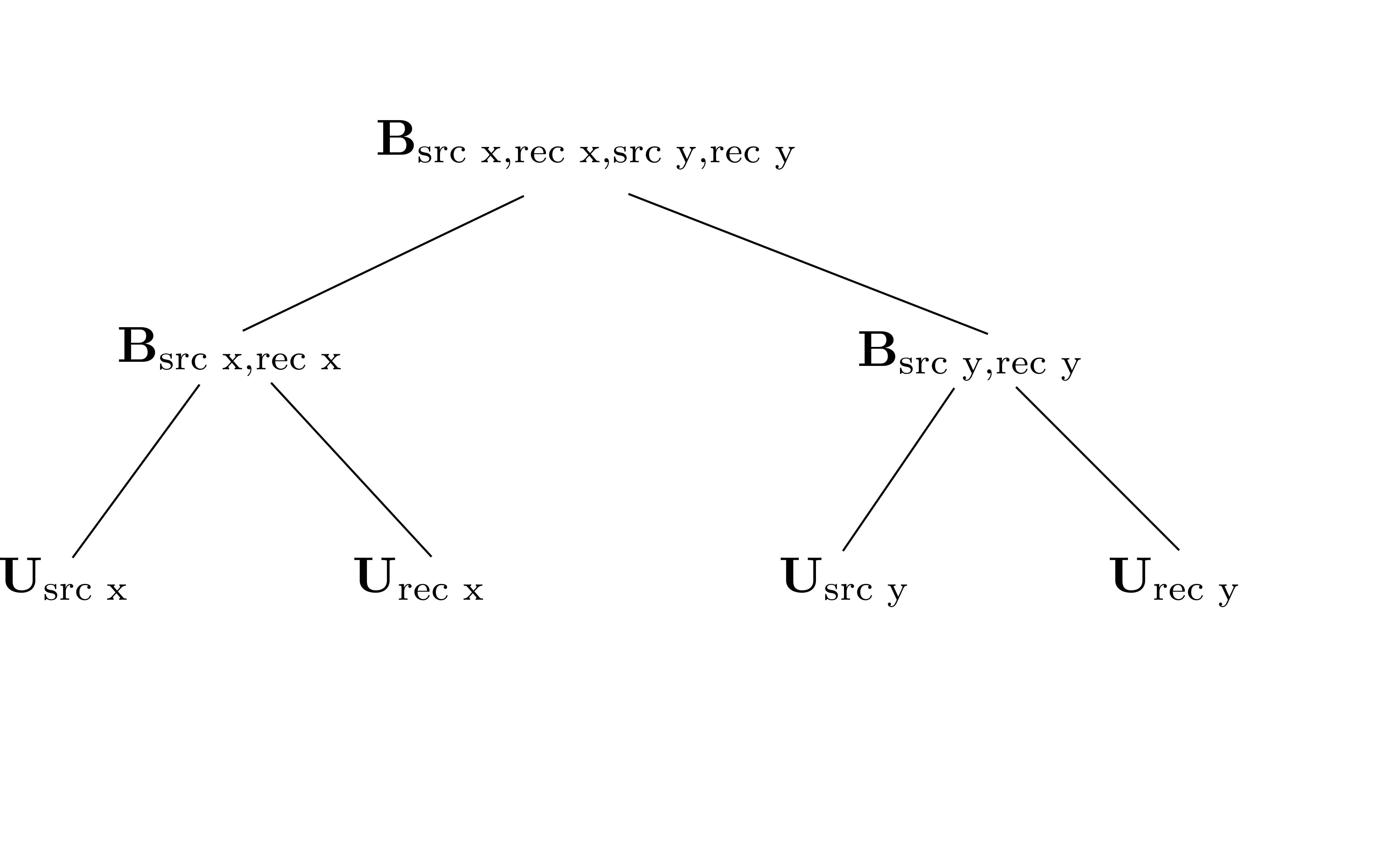
It is critical to note that the organization of the tensor has a major impact on its low-rank behaviour. In the seismic context, we permute our data from the typical or canonical organization (source x, source y, receiver x, receiver y) into a non-canonical organization (source x, receive x, source y, receiver y), which results in faster decaying singular values for associated matricizations (Da Silva and Herrmann, 2015; A. Aravkin et al., 2014). The dimension tree associated to this organization is shown in Figure 2. From the perspective of low-rank reconstruction, considering randomly missing sources or receivers in the non-canonical ordering leads to growth of the singular values in the corresponding matricizations of the tensor, leading to more favourable recovery conditions as explored in (Kumar et al., 2015). The resulting HT parameters are indexed as \[ \begin{equation} \begin{aligned} &U_{t} \in \mathbb{C}^{n_t \times k_t} \quad &t = \text{src x, src y, rec x, rec y} \\ &B_{t} \in \mathbb{C}^{k_{t_l} \times k_{t_r} \times k_t} \quad &t = \text{ (src x, rec x), (src y, rec y),} \\ & &\text{ (src x, rec x, src y, rec y) }, \end{aligned} \label{htparams} \end{equation} \] where \(n_t, k_t\) corresponds to the dimensions and ranks indexed by the label \(t\), respectively.

Given fully sampled seismic data in the non-canonical organization, one can truncate the full tensor to HT form via the algorithm in (Tobler, 2012), given a prescribed error tolerance and maximum inner rank. In the more realistic case when we have subsampled data, we can use the algorithm described in (Da Silva and Herrmann, 2015) to recover the full data volume by solving \[ \begin{equation} \min_{x} \| \mathcal{A} \phi(x) - b \|_2^2. \label{HTinter} \end{equation} \] Here \(x\) is the vectorized set of HT parameters \((U_t, B_t)\) from \(\eqref{htparams}\), \(\phi\) maps \(x\) to the fully-expanded tensor \(\phi(x)\), \(\mathcal{A}\) is the subsampling operator, and \(b\) is our subsampled data. This algorithm can interpolate each 4D monochromatic slice quickly and efficiently as it does not compute SVDs on large matrices.

On-the-fly extraction of shot/receiver gathers

Irrespective of our sampling regime, once we have a representation of our data volume in the HT format, we can greatly reduce the computational costs of working with our data. In order to make use of the data directly in its compressed form, we present a method for extracting a shot (or receiver) gather at a given position \((i_x, i_y)\) directly from the compressed parameters. We use Matlab colon notation \(A(i,:)\) to denote the extraction of the \(i^{\text{th}}\) row of the matrix \(A\), and similarly for column extraction. The common shot gather can be reconstructed by computing \[ \begin{equation} \begin{aligned} &U_{src x,rec x} = U_{src x}(i_x,:) \times_1 U_{rec x} \times_2 B_{src x,rec x} \\ &U_{src y,rec y} = U_{src y}(i_y,:) \times_1 U_{rec y} \times_2 B_{src y,rec y} \\ &D_{i_x,i_y} = U_{src x,rec x} \times_1 U_{src y,rec y} \times_2 B_{src x,rec x,src y,rec y} \end{aligned} \label{slicing} \end{equation} \] Most importantly, all the computations in Equation \(\eqref{slicing}\) can be efficiently implemented with Kronecker products or matrix-vector products, outlined in Algorithm 1. Note that the intermediate quantities can be constructed through efficient multilinear products and are much smaller than the ambient dimensionality.

 Input: Source position \(i_x\) and \(i_y\), and dimension tree
 1. Extract the vector \(u_{src x}\) from the matrix \(U_{src x}(i_x,:)\)
 2. Multiply \(B_{src x,rec x}\) along the \(k_{src x}\) dimension with the vector \(u_{src x}\) (in the sense of Definition 2)
 3. Multiply the matrix obtained from step \(2\) along the \(k_{rec x}\) dimension (second dimension) with \(U_{rec x}\), resulting in a matrix \(U_{srcx,recx}\) of size \(n_{rec x}\times k_{(src x, rec x)}\)
 4. Repeat steps \(1, 2, 3\) along the \(y\) coordinate to obtain the matrix \(U_{srcy,recy}\) of size \(n_{rec y} \times k_{(src y, rec y)}\)
 5. The product \(U_{srcx,recx} B_{srcx,recx} U_{srcy,recy}^T\) results in the final shot gather

Experiments & Results

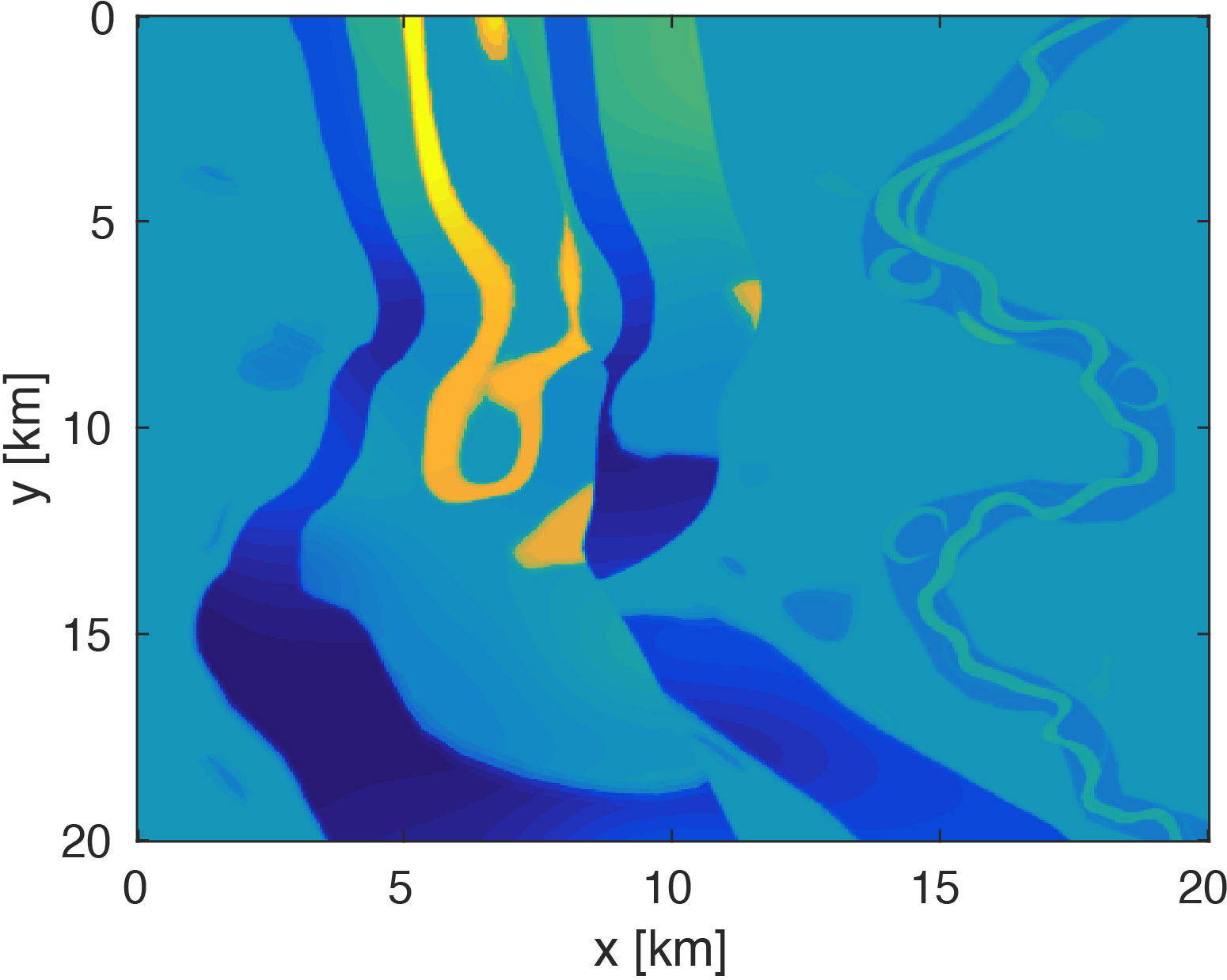
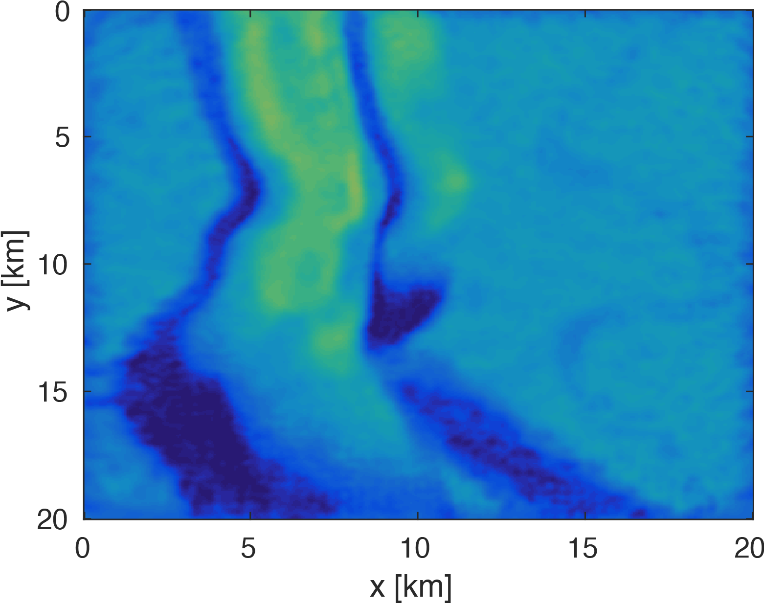
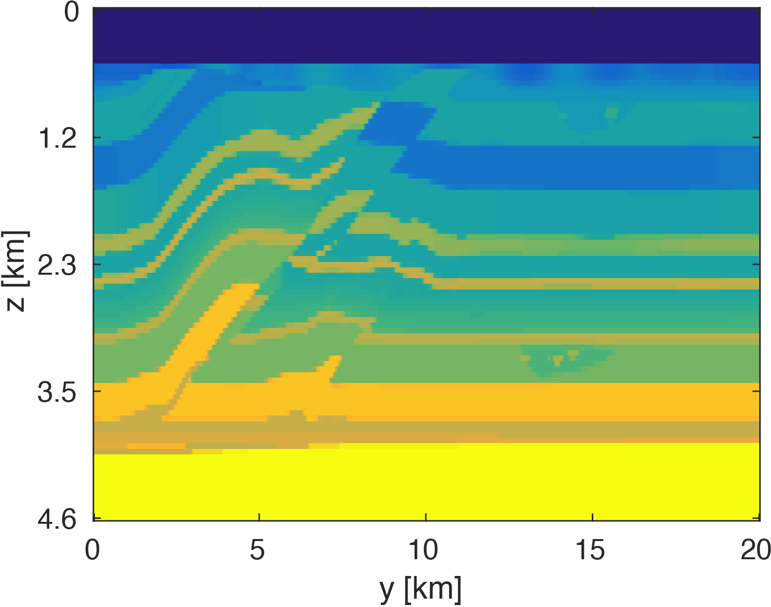
To demonstrate that our method significantly reduces memory costs of working with the data volume, we consider full-waveform inversion on the SEG/EAGE 3D Overthrust velocity model. This \(20km \times 20km \times 5km\) velocity model, discretized on a \(50m\) grid in each direction, contains structurally complex areas such as fault belts and channels. We modify this model by adding a \(500m\) water layer on top.

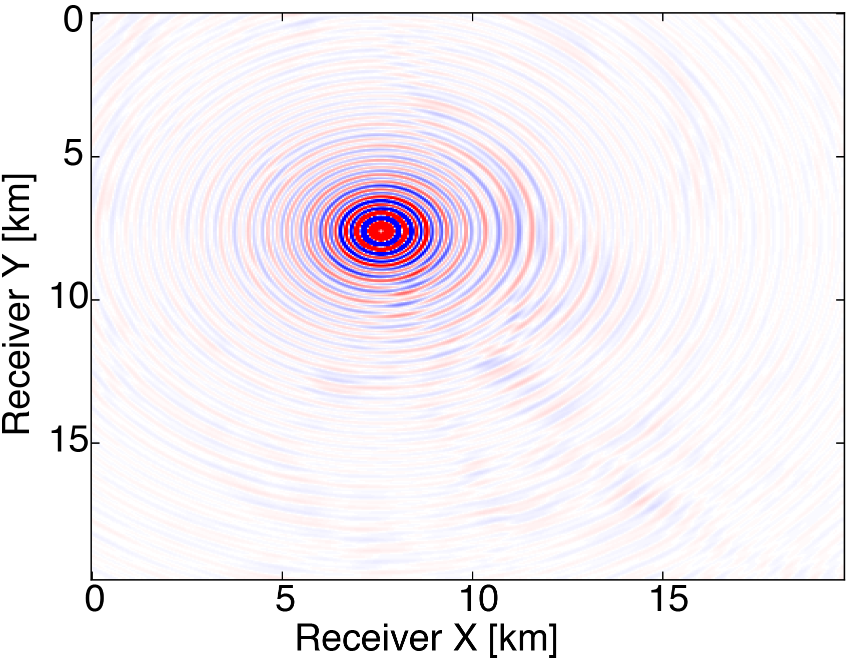
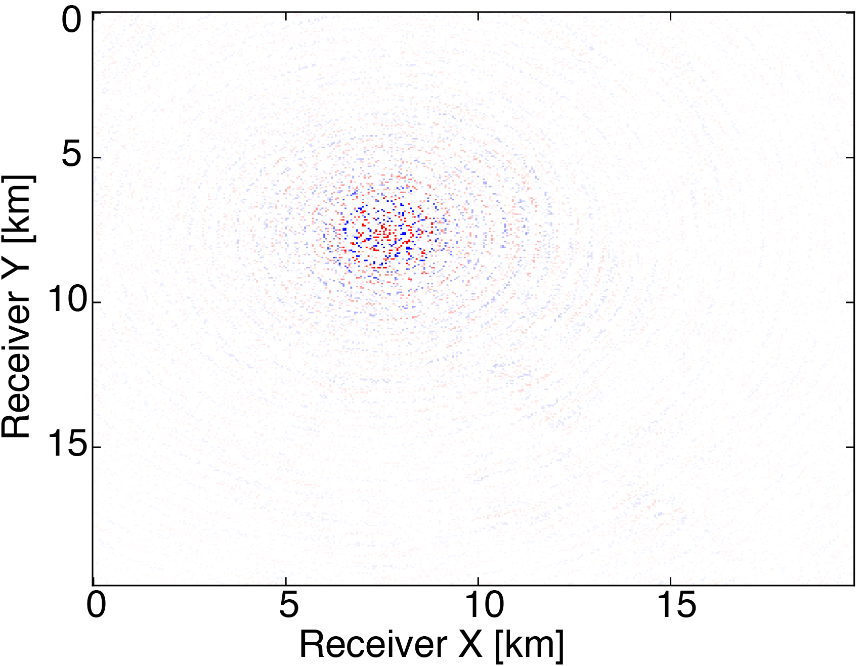
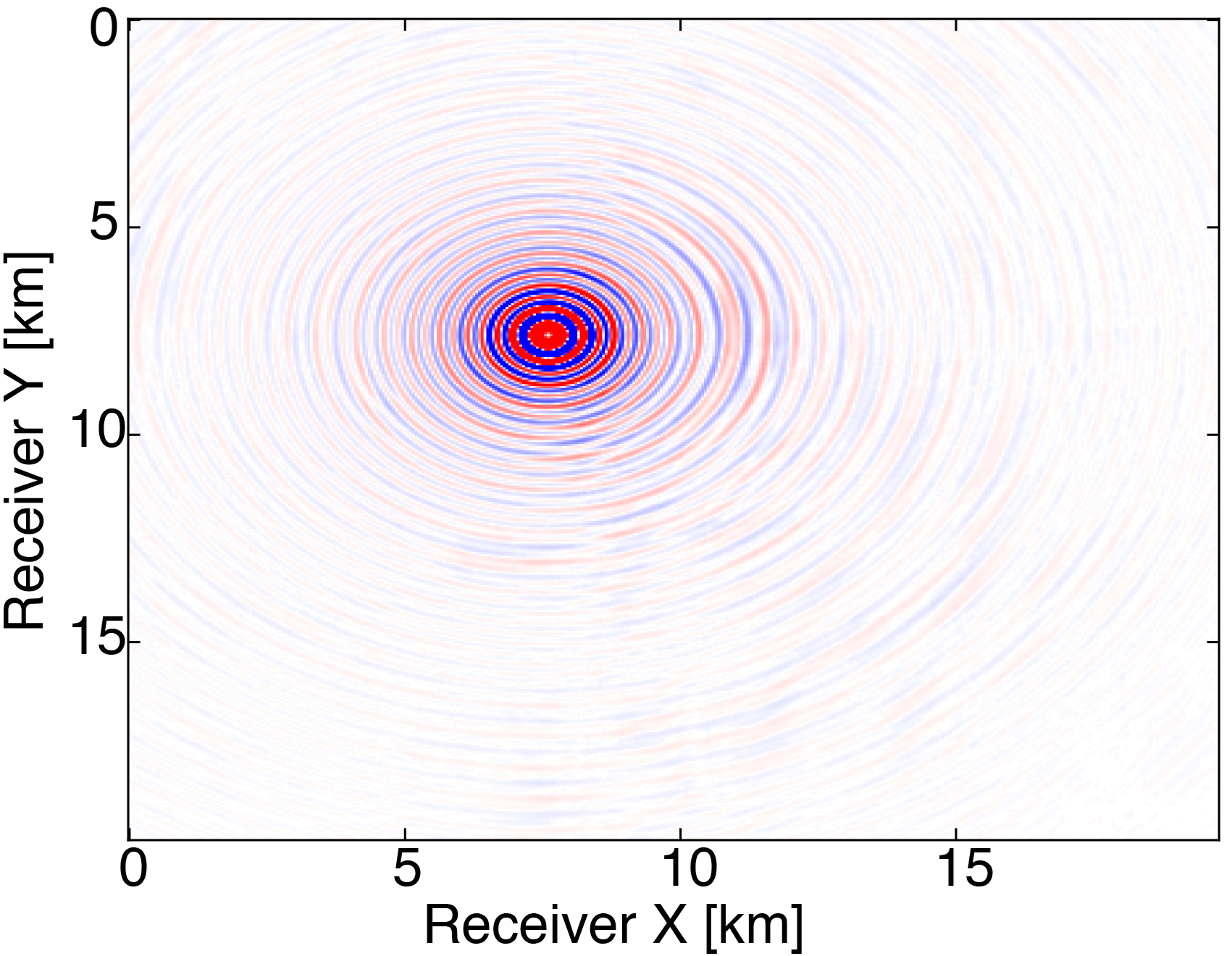
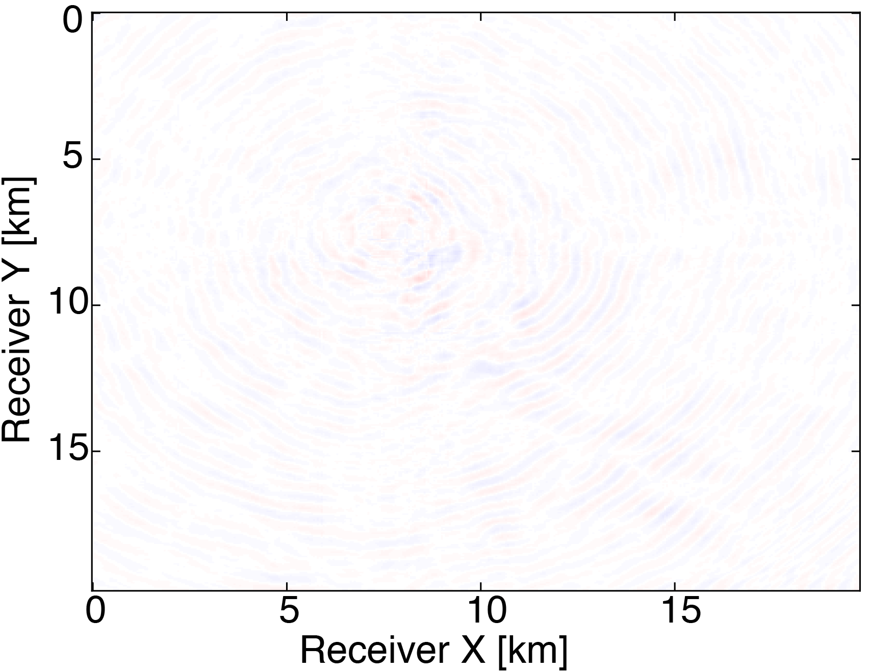
We generate our data from \(4\) frequencies between \(3Hz\) and \(6Hz\) with spacings of \(1Hz\) using a \(50 \times 50\) source grid with \(400m\) spacing and a \(396 \times 396\) receiver grid with \(50m\) spacing on the ocean bottom. The size of each frequency slice is roughly \(5.8GB\). From the full data, we randomly remove \(80 \%\) of receivers from each frequency slice. We then are able to obtain our compressed data volume for each monochromatic slice by interpolating in the HT format. Figure 3 demonstrates the successful interpolation of the data volume from a high level of missing data, resulting in shot-gathers that are simple to extract with \(\eqref{slicing}\).

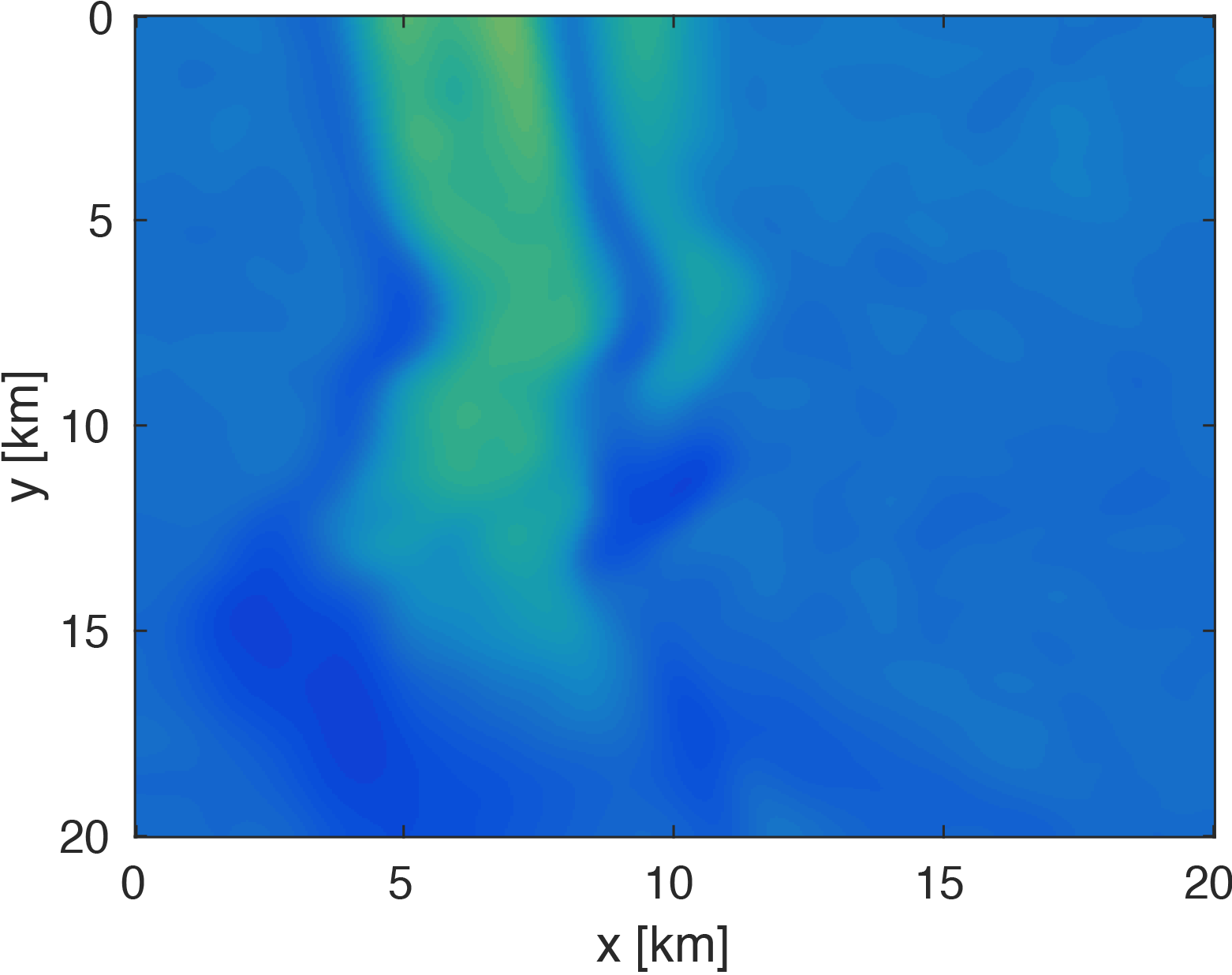
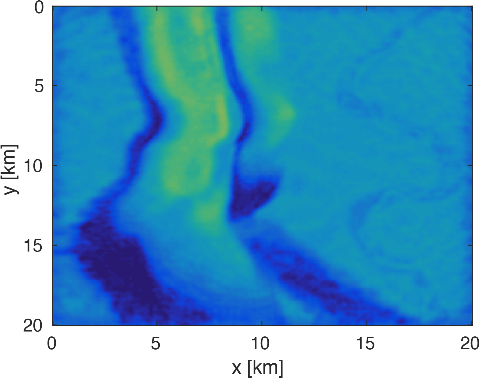
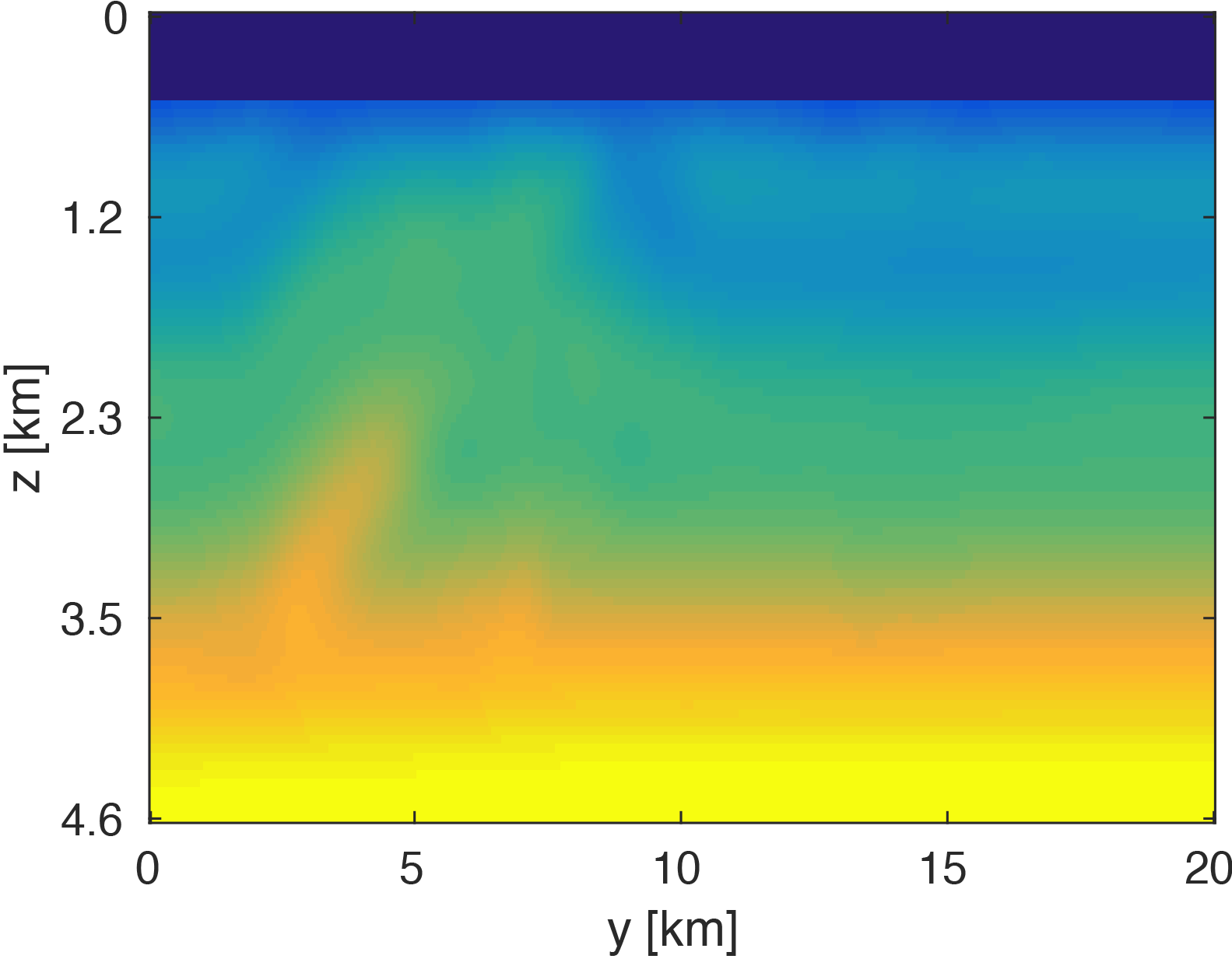
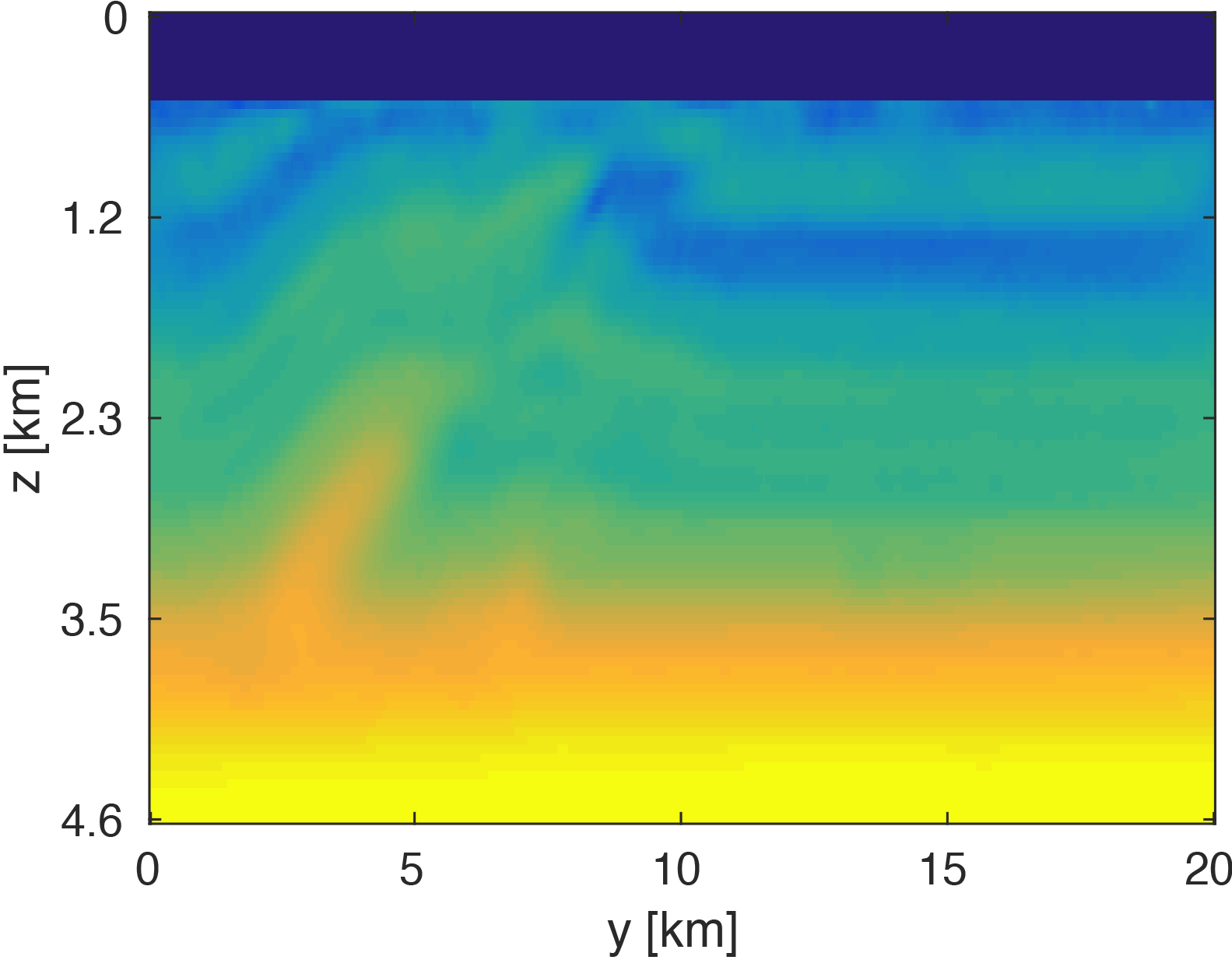
The modeling code we employ is WAVEFORM, which is a Helmholtz inversion framework written primarily in Matlab (Da Silva and Herrmann, 2016). Considering the large number of sources in these experiments, we use a stochastic optimization algorithm that works on randomly subsampled subsets of shots rather than using all the shots at each iteration, which reduces the number of PDEs to be solved at a given iteration. For each subset of shots, we partially minimize the resulting least-squares objective function with the LBFGS algorithm with bound constraints, i.e. minimum and maximum allowed velocities (Schmidt et al., 2009). We invert a single frequency at one time using \(50\) nodes with \(8\) Matlab workers running for each, where each node has \(20\) CPU cores and \(256GB\) of RAM. We run the 3D FWI experiments for both the full data and compressed HT data recovered from interpolation, fixing the total number of PDEs solved. In this case, we design an interface to our stochastic inversion algorithm that allows the algorithm to automatically determine the shot gather indices required at a given iteration, which are subsequently generated by \(\eqref{slicing}\). Figure (4) and (5) show inversion results for both full data and compressed data. Despite working with heavily subsampled initial data, the interpolation algorithm is able to accurately estimate the entire data volume and the compressed parameters are used to successfully invert the velocity model at a greatly reduced memory cost. In this case, the data volume sizes are reduced by over \(90\%\), with little visual difference in the final inversion results.

Conclusions & Discussion

In this paper, we propose an approach to represent our large-scale 5D data set in terms of its low-rank tensor parametrization. This approach is suitable for when the data is fully sampled or missing randomly distributed sources or receivers. Rather than explicitly forming the full data volume, we utilize the data directly in its compressed form, giving query-based access to the full volume. This approach extracts any common shot or receiver gathers on-the-fly, making its code easily embedded into other processing frameworks such as 3D FWI. The proposed approach is computationally and memory efficient without degrading subsequent results.

The techniques outlined in this work have the potential to substantially reduce data communication costs in distributed wave-equation based inversion. In a parallel environment, we can cheaply store a compressed form of the full data volume at a given frequency on every node. This technique also lends itself to generating simultaneous shots on-the-fly in a similar manner to Algorithm (1), without the associated data communication costs one would incur from distributing the full data volume over the source dimension. The very high compression ratios (greater than \(90\%\) in this example) are particularly enticing for low frequency full waveform inversion.

Acknowledgements

This research was carried out as part of the SINBAD II project with the support of the member organizations of the SINBAD Consortium. The authors wish to acknowledge the SENAI CIMATEC Supercomputing Center for Industrial Innovation, with support from BG Brasil, Shell, and the Brazilian Authority for Oil, Gas and Biofuels (ANP), for the provision and operation of computational facilities and the commitment to invest in Research & Development.