Fast sparsity-promoting least-squares migration with multiples in the time domain

Summary:

Based on the latest developments of research in inversion technology with optimization, researchers have made significant progress in the implementation of least-squares reverse-time migration (LS-RTM) of primaries. In Marine data however, these applications rely on the success of a pre-imaging separation of primaries and multiples, which can be modeled as a multi-dimensional convolution between the vertical derivative of the surface-free Green’s function and the down-going receiver wavefield. Instead of imaging the primaries and multiples separately, we implement the LS-RTM of the total down-going wavefield by combining areal source injection and linearized Born modelling, where strong surface related multiples are generated from a strong density variation at the ocean bottom. The advantage including surface related multiples in LS-RTM is the extra illumination we obtain from these multiples without incurring additional computational costs related to carrying out multi-dimensional convolutions part of conventional multiple prediction procedures. Even though we are able to avert these computational costs, our approach shares the large costs of LS-RTM. We reduce these costs by combining randomized source subsampling with our sparsity-promoting imaging technology, which produces artifact-free, high-resolution images, with the surface-related multiples migrated properly.

Introduction

By fitting the modeled primaries to observed primaries in the least-squares sense, least-squares reverse-time migration (LS-RTM, (Guitton et al., 2006)) can remove the imprint of the source wavelet, limited aperture, and other amplitude effects on migrated images. Since minimizing the \(\ell_2\)-norm on the data residual attempts to invert a highly overdetermined but inconsistent system, resulting images often suffer from overfitting. One possible way to remove these artifacts is to impose some sort of regularization on to the original LS-RTM formulation. Aside from imaging artifacts associated with possible overfitting, LS-RTM is also computationally prohibitively expensive withstanding its widespread adaptation. Motivated by ideas from Compressive Sensing (Donoho, 2006), Herrmann and Li (2012) proposed to solve the expensive overdetermined and inconsistent system of LS-RTM by solving a series of much smaller and therefore much cheaper randomized subproblems. Thanks to this randomized subsampling, we are able to carry out sparsity-promoting LS-RTM at the cost of roughly one-to-three passes through the data. However, the resulting images remained somewhat noisy, a well-known by product of stochastic optimization methods where different subsets of shots are used during each iteration. By replacing the \(\ell_1\) norm objective by an elastic net, as proposed by Lorenz et al. (2014) in the field of online Compressive Sensing, these remaining noisy artifacts can be removed as shown by F. J. Herrmann et al. (2015). Following this work, Yang et al. (2016) implemented this linearized Bregman method in the time domain including on-the-fly source estimation with variable projection.

So far, this work mostly involved imaging of primaries only. For (shallow) Marine data, this assumption requires separation of primaries from the total down-going wavefield, which includes surface-related multiples. One way to separate the primaries is to consider the surface-related multiples elimination (SRME) relation (Verschuur et al., 1992), which models multiples as a multi-dimensional convolution between the vertical derivative of the surface-free Green’s function and the total down-going wavefield. While this relation has resulted in technologies such as SRME and Estimation of Primaries by Sparse Inversion ((EPSI), Lin and Herrmann, 2013) that mitigate the adverse effects of surface-related multiples successfully, it is computationally very expensive because it involves multi-dimensional convolutions that correspond to dense matrix-matrix multiplies. Also, SRME requires the sources to be co-located with the receivers, which is can be expensive as well. Besides the computational cost, SRME struggles to estimate the source wavelet and therefore the shape of the recovered primaries may get distorted, especially in shallow water acquisitions. EPSI on the other hand, maps the multiples to primaries, which offers the potential to use these multiples the help with illumination of the subsurface. Lu et al. (2015) and also Tu and Herrmann (2015) used the fact that the bounce points of surface-related multiples can be considered as secondary sources to improve migrated images. Lu et al. (2015) did this by replacing RTM’s cross-correlation based imaging condition by a deconvolution. While the results of this later approach have been spectacular (Lecerf et al., 2015), deconvolution imaging conditions can lead to unwanted crosstalk caused by interference between different orders of multiples.

By integrating the SRME relationship into sparsity-promoting LS-RTM, Tu and Herrmann (2015) was able to properly model surface-related multiples resulting in an inversion procedure where surface-related multiples are mapped to imaged reflectors. His main contribution was that integrating the SRME relation into LS-RTM simply corresponds to adding the down-going wavefield as an areal source. As such Tu and Herrmann (2015) arrived at a result where the multi-dimensional convolutions of EPSI are carried out by the wave-equation solver while this formulation also no longer requires co-location of sources and receivers during acquisition. While this work (Tu and Herrmann, 2015) has resulted in high-quality multiple-free images, it relied on an unnatural strong perturbation in the velocity to generate realistic surface-related multiples in the water column. We remove this problem by including density variations at the ocean bottom into our time-doman formulation (Yang et al., 2016). Because our time-stepping formulation is based on Devito (Lange et al., 2016) — a just in time compiler for stencil-based finite-difference codes — we envision that the proposed approach can readily be extended to 3D seismic.

Our abstract is organized as follows. First, we describe multiples prediction with the SRME and formulate the areal source injection into our linearized Born modelling operator mapping velocity and density perturbations to linearized data. Next, we derive an optimization scheme for LS-RTM using a mixed \(\ell_1\)-\(\ell_2\)-norm objective function with areal source included. We solve this problem with linearized Bregman. The experiments are set up with the synthetic SIGSBEE2A model (Paffenholz et al., 2002), where the inversion results of total down-going wavefield with and without areal source injection are compared.

Theory

SRME and areal source

The SRME relation (Verschuur et al., 1992) forms the foundation of most multiples separation methods since it relates the vertical derivative of the surface-free Green’s function and the downgoing wavefield to the total upgoing wavefield—i.e. we have \[ \begin{equation} \mathcal{P}_i = \mathcal{G}_i(\mathcal{Q}_i + \mathcal{R}_i\mathcal{P}_i), \label{SRME} \end{equation} \] where the subscript \(i \in \Omega=[1 \dots n_f]\) with \(n_f\) the total number of discretized frequencies. The matrix\(\mathcal{P}_i\) stands for the total up-going wavefield at the surface with \(n_s\) common-shot gathers in its columns and \(n_r\) common-receiver gathers in its rows. Note that this data matrix \(\mathcal{P}_i\) does not include direct waves. The matrix\(\mathcal{G}_i\) denotes the surface-free dipole Green’s function organized in a similar fashion. The matrix \(\mathcal{Q}_i\) represents the down-going point source wavefield, \(\mathcal{R}_i\) is the reflectivity at surface, and normally is \(-1\). The whole term \(\mathcal{R}_i\mathcal{P}_i\) acts as an areal source wavefield, which when multiplied by \(\mathcal{G}_i\) produces the total upgoing wavefield including surface-related multiples.

Tu and Herrmann (2015) incorporated the above SRME relation into an expression for linearized modelling \[ \begin{equation} \begin{aligned} \mathcal{P}_i & \approx \ \nabla \mathcal{F}_i [\vector{m}_0, \delta \vector{m}; \mathcal{I}] (\mathcal{Q}_i - \mathcal{P}_i)\\ & = \nabla \mathcal{F}_i [\vector{m}_0,\delta \vector{m}; \mathcal{Q}_i - \mathcal{P}_i] \\ & = \nabla \mathcal{F}_i [\vector{m}_0; \mathcal{Q}_i-\mathcal{P}_i] \delta \vector{m}. \end{aligned} \label{model_arealS} \end{equation} \] In this expression, \(\nabla \mathcal{F}_i\) represents the vertical deriavtive of linearized Born modelling, which is linear in the model perturbation \(\delta \vector{m}\) and the impulsive source array \(\mathcal{I}\). When the background model \(\vector{m}_0\) is kinetically correct, \(\nabla \mathcal{F}_i\) is a good approximation of the Green’s function \(\mathcal{G}_i\). By using fundamental properties of Green’s function the third expression in Equation \(\eqref{model_arealS}\) replaces the expensive convolutions in the first expression by including the downgoing wavefield as an areal source.

In time domain, the relationship \(\ref{model_arealS}\) can be formulated directly as \[ \begin{equation} \vector{P} \approx \nabla \vector{F} [\vector{m}_0; \vector{Q} - \vector{P}] \delta \vector{m}, \label{model_arealS_time} \end{equation} \] where \(\vector{P}\), \(\vector{Q}\), \(\nabla \vector{F}\) denote the corresponding operators in the time domain.

To generate realistic surface-related multiples in the water column, we introduce density variations\(\boldsymbol{\rho}\) at the ocean bottom. Equation \(\ref{model_arealS_time}\) now becomes \[ \begin{equation} \begin{aligned} \vector{P} & \approx \nabla \vector{F}_{\vector{m},\boldsymbol{\rho}}[\vector{m}_0, \boldsymbol{\rho}_0; \vector{Q}-\vector{P}] \left[ \begin{matrix} \delta \vector{m}\\ \delta \boldsymbol{\rho}\\ \end{matrix} \right]\\ & \approx \nabla \vector{F}_{\vector{m}}[\vector{m}_0, \boldsymbol{\rho}_0; \vector{Q}-\vector{P}] (\delta \vector{m} + \delta\vector{m}^{\prime}). \end{aligned} \label{model_arealS_time_density} \end{equation} \] In this expression, \(\nabla \vector{F}_{\vector{m}, \boldsymbol{\rho}}[\vector{m}_0,\boldsymbol{\rho}_0;\vector{Q}-\vector{P}]\) corresponds to linearized Born modelling with respect to perturbations in the velocity and density, respectively. The operator \(\nabla \vector{F}_{\vector{m}}[\vector{m}_0,\boldsymbol{\rho}_0;\vector{Q}-\vector{P}]\) corresponds to linearized Born modelling with respect to velocity changes only. When we linearize the wave equation with respect to a constant density, Born modelling for density variations equals Born modelling for velocity variations, a property we used in Equation \(\ref{model_arealS_time_density}\), where \(\delta\vector{m}^{\prime}\) is the density induced “velocity” perturbation at the Ocean bottom. By including this additional term, we are able to model realistic surface-related multiples in the water column without relying on unrealistic and numerical problems inducing velocity perturbations. Note, that we assume the density to be constant throughout the remainder of the model so the migrated amplitudes should be interpreted as impedance perturbations in cased where there are strong variations of the density in the subsurface.

Sparsity-promoting LS-RTM with areal source injection

Tu (2015) demonstrated that sparsity-promoting LSRTM leads to artifact-free high-resolution images. When using the linearized Bregman method with source subsampling, we obtain these images by solving \[ \begin{equation} \begin{aligned} \min_{\vector{x}} \ & \lambda \Vert\vector{x} \Vert_1 + \frac{1}{2} \Vert\vector{x} \Vert^2_2 \\ & \text{subject to} \ \sum_{j} \Vert \nabla \vector{F}_{j}( \vector{m}_0, \vector{\rho}_0, \vector{Q}_j - \vector{P}_j) \vector{C}^T \vector{x} - \vector{P}_{j}\Vert_2 \leq \sigma, \end{aligned} \label{obj} \end{equation} \] where \(\vector{x}\) represents the curvelet coefficient vectors for the velocity perturbation \(\delta\vector{m} + \delta\vector{m}^{\prime}\). \(\Vert \cdot \Vert_1\) and \(\Vert \cdot \Vert_2\) stand for \(\ell_1\) and \(\ell_2\) norms, respectively. The sum runs over all shots, \(\sigma\) is the two-norm of the noise. For \(\lambda\) large enough, the solutions of this problem corresponds to the solution of problems with a \(\ell_1\)-norm objective. We refer to F. J. Herrmann et al. (2015) foer a discussion on the role of the thresholding parameter \(\lambda\).

We summarize pseudo code to solve problem \(\ref{obj}\) in Algorithm 1.

In Algorithm 1, \(\mathbb{P}_{\sigma}\) projects the residual onto a noise \(\sigma\) related \(\ell_2\)-norm ball. In our LS-RTM case, the threshold \(\lambda\) should chosen according to the maximum of \(\vector{z}_k\) to let elements of \(\vector{z}_k\) enter to solution \(\vector{x}_k\).

Numerical Experiments

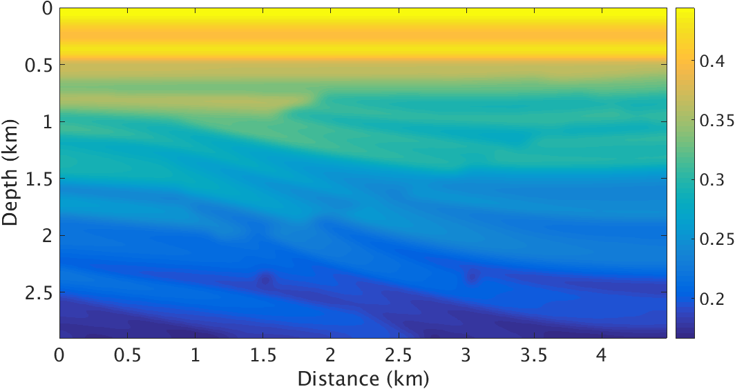
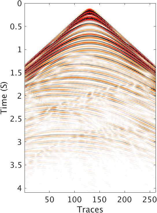
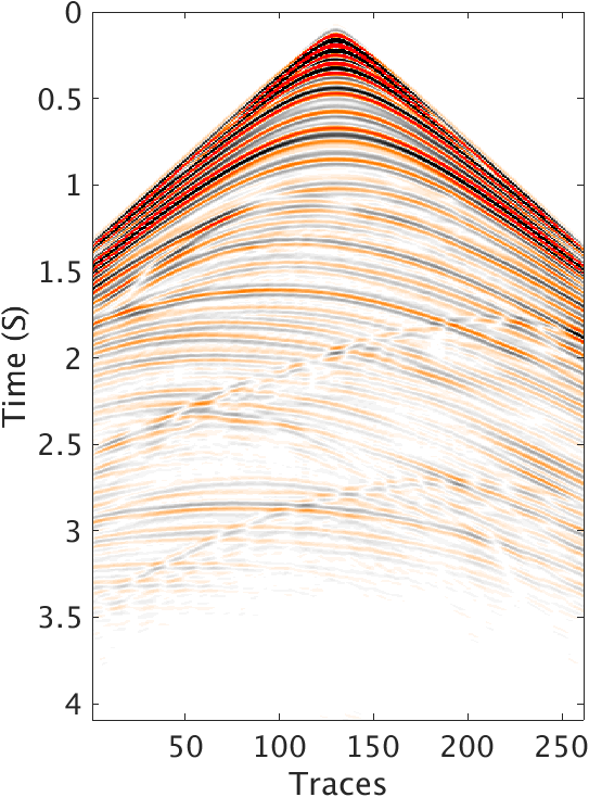
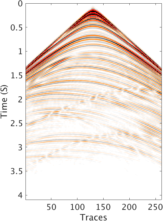
To test the performance of this method, we conduct the experiments based on a shallow water model modified from SIGSBEE2A model shown in Figure 1, which is discretized with grid size of \(5\mathrm{m}\), totally \(4.15\mathrm{km}\) deep and \(4.48\mathrm{km}\) wide. The water layer is roughly \(100\mathrm{m}\) deep. The background velocity \(\vector{m}_0\) is smoothed from the true model and is kinematically correct. The density model is converted from velocity background model by the Gardner relation in the sedimental layers, and the value for water layer is constant 1. So in the true density model there is only sharp perturbation near the ocean bottom. We compare the images inverted with all the reflection data with and without our method. We use a Ricker wavelet centered at \(15 \mathrm{Hz}\) as source wavelet and record the data for 4.0 seconds. The \(261\) shots and \(261\) receivers are spread over the top of the model from \(290\mathrm{m}\) to \(4190\mathrm{m}\) in the horizontal direction, with 15m spacing at the depth of \(20\mathrm{m}\). The data was generated with iWave, and inverted with Devito. Figure 2 shows one shot record after receiver-side deghost and extrapolation to surface, indicating the strong multiples inside. In LSRTM, we rerandomize data subset of 12 shots in every iteration, roughly \(5\%\) of the total data. We totally run one data pass in inversion. We also use the pre-conditioners mentioned in Yang et al. (2016) to accelerate the inversion.

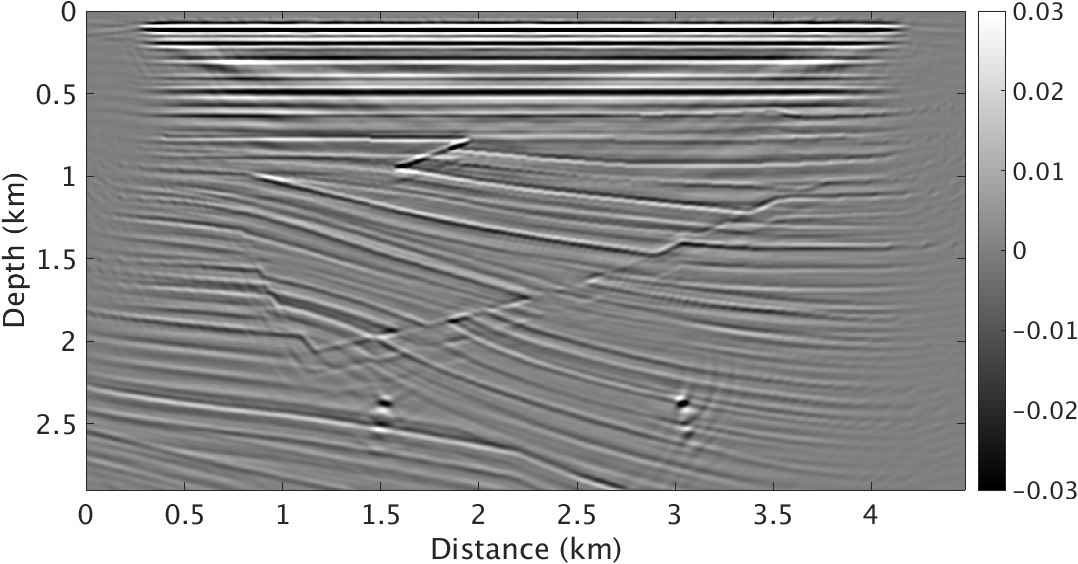
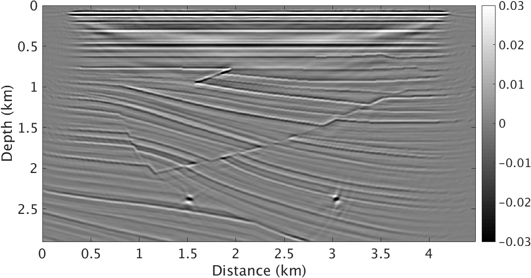
The image we get by inverting all the reflection data directly with absorbing surface and dipole sources has interference of some shadows of the relative shallower layers. These shadows are harder to identify than those in deep water case and they are almost as strong as true layer interfaces. Figure 3a clearly shows these shadows, which will be wiped out by areal source injection, shown in Figure 3b. Figure 3b is not perfect, especially around the area of these two refraction points near \(2.5 \mathrm{km}\) and near the ocean bottom. The remaining weak shadows near the ocean bottom are due to the fact that we invert the density perturbation into a velocity perturbation. Figure 4 clearly shows the difference between the images with and without areal source injection. By comparing the linearized data of only dipole point source Born modelling with the recovery model perturbations, it’s clear that the shot record generated without our methods still contains multiples. While, multiples in the shot record generated with the recovery model perturbation of our method are pressed a lot.

Conclusions

In this work, we image primaries and multiples jointly by sparsity promoting LS-RTM using an areal source injection that included the downgoing wavefield and a time-domain formulation of the linearized Bregman method. With this methodology, we remove imaging artifacts related to the presence of surface-related multiples induced by a shallow layer. These types of multiples are difficult to remove by methods such as SRME. Instead of removing these multiples, we image them by including the downgoing wavefield in the Born modeling operator. In this wat, we even take advantage of extra illumination that stems from these multiples, whose bounce points at the surface can be considered as additional insonifying secondary sources. For this reason, the image obtained by our method is better illuminated in the shallow parts of the sedimental layers. The cost of this method is same as the cost of inverting primaries, one RTM computation roughly. Because our work uses recently developed just-in-time compiler technology for time-stepping finite difference, we are in a good position to extend the presented approach to 3D seismic.

Acknowledgements

We would like to acknowledge Mathias Louboutin and Philipp Witte for the platform work of Devito and Julia interface for the time stepping finite difference modeling code. We also thank the authors of iWave. This research was carried out as part of the SINBAD project with the support of the member organizations of the SINBAD Consortium.