High resolution fast microseismic source collocation and source time function estimation

Introduction

There has been increased attention towards unconventional reservoirs in last couple of decades. Unconventional reservoirs require some kind of stimulation in the form of hydraulic fracturing to make them economically viable for production by connecting weakly connected oil & gas traps through the fractures. For production purposes and to prevent any kind of hazardous situations (e.g. interference of these fractures with pre-existing wells and faults) it is extremely important to estimate the fracture locations accurately together with other attributes such as source time function, stress orientation along these fractures, etc. Among all the available methods, microseismic based methods provide most accurate way to estimate the above mentioned attributes of fractures (Maxwell, 2014).

As fractures caused by hydraulic fracturing propagate through the subsurface rocks, they generate microseismic waves that are recorded by receivers along the surface or receivers along monitor wells. The recorded microseismic data contains information about the source attributes such as source location, source time function, source mechanism etc. One exploits this microseismic data to find out different source attributes, which is extremely helpful for drilling decisions, hazard prevention etc.

Traditional methods based on travel time inversion require travel time picking and identification of phases such as P and S wave components (Thurber and Engdahl, 2000; Waldhauser and Ellsworth, 2000). These methods estimate the location but not the source time function. Recently developed methods based on imaging (McMechan, 2010; Gajewski and Tessmer, 2005; Sun et al., 2015; Nakata and Beroza, 2016) do not require travel time picking but only estimate source location, again without the source time function.

Kaderli et al. (2015) suggested a FWI based method to estimate both source location and source time function in an alternating fashion. H. Wang and Alkhalifah (2016) proposed to use FWI to invert for source location, source time function and the velocity model in an alternating fashion. Both of these works assumed that the spatial and temporal component of a source is separable. Moreover, they showed results only for a single source. However, in real life there can be more than one microseismic sources. Sharan et al. (2016) showed that in order to use FWI with the assumption of separable source location and source time function, one need to know the number of sources beforehand. For hydraulic fracturing scenario the knowledge of number of microseismic sources is not a trivial problem. Also, FWI based method suggested by Kaderli et al. (2015) performs poorly when both the source location and source time function are unknown, which is mostly the situation for real life scenario.

In Sharan et al. (2016), the authors exploited the fact that wave equation itself is an excellent sparsity promoting transform to simultaneously estimate the microseismic source location & source time function without any prior assumptions about the number of sources or any initial guess about the source location and source time function. They used the Linearized Bregman algorithm to jointly estimate the microseismic source location & source time function. Although, this algorithm is simple to implement, it suffers from slow convergence because of the 1st order convergence. As each iteration of the algorithm required two PDE solves (Forward and adjoint wave-equation solve in time domain), using the Linearized Bregman algorithm can be too expensive for a complex problem. Huang et al. (2013) and Wotao Yin (2010) showed that the Linearized Bregman algorithm is equivalent to solving a gradient descent of the dual problem and therefore they proposed to use a Limited memory BFGS (Liu and Nocedal, 1989) kind of method to accelerate the convergence of original Linearized Bregman algorithm from \(1^{st}\) order to \(2^{nd}\) order of convergence. Motivated by this idea, in this work, we propose to use Linearized Bregman algorithm with LBFGS to attain faster convergence for the joint microseismic source-collocation and source time function estimation problem. We also extend our proposed method to the situations involving 2.5 D wave propagation instead of 2D wave propagation. We then demonstrate the effectiveness of our method for complex geology and closely spaced sources with different source-time functions with different dominant frequencies.

Methodology

Given a sufficiently accurate velocity model, Sharan et al. (2016) exploited the fact that the wave equation acts as a sparsity promoting “transform” by focusing wavefields on their correct source locations. Assuming sources are localized in space and have finite energy along time, Sharan et al. (2016) proposed to solve \[ \begin{equation} \min_{\vector{U}} \quad \|\mathcal{A}[\vector{m}]\ (\vector{U})\|_{2,1} \quad \text{s.t.} \quad \|\mathcal{P}(\vector{U}) - \vector{d}\|_2 \leq \epsilon. \label{eqMoti} \end{equation} \] Equation \(\ref{eqMoti}\) aims to minimize the \(\|.\|_{2,1}\) norm of action of finite difference time stepping operator \(\mathcal{A}[\vector{m}]\), parametrized by squared slowness \(\vector{m}\), on spatio-temporal wavefield \(\vector{U}\) under the condition that receiver restriction operator \(\mathcal{P}\) restricts the wavefield \(\vector{U}\) to fit the observed microseismic data \(\vector{d}\) within \(\epsilon\), the two-norm of noise level. The \(\|.\|_{2,1}\) norm was used to exploit the fact that sources have finite energy along time but are sparse along space. The operators \(\mathcal{A}[\vector{m}] (\vector{U})\) and \(\mathcal{P}(\vector{U})\) are linear in terms of wavefield \(\vector{U}\). Sharan et al. (2016) proposed to make the above optimization problem more tractable by a simple change of variable \(\vector{Q}=\mathcal{A}[\vector{m}] (\vector{U})\), where \(\vector{Q}\) is a matrix containing spatial temporal distribution of all the sources—i.e. the \((i,j)\) entry in \(\vector{Q}_{i,j} = {q}(x_i,t_j)\). So equation \(\ref{eqMoti}\) becomes: \[ \begin{equation} \min_{\vector{Q}} \quad \|\vector{Q}\|_{2,1} \quad \text{s.t.}\quad\|\mathcal{F}[\vector{m}] (\vector{Q}) - \vector{d}\|_2 \leq \epsilon, \label{eqBPDN} \end{equation} \] where \(\mathcal{F}[\vector{m}]=\mathcal{P}{\mathcal{A}[\vector{m}]}^{-1}\) is the forward modeling operator which is a linear operator in terms of \(\vector{Q}\) . Equation \(\ref{eqBPDN}\) is similar to the classic basis pursuit denoising (BPDN) problem. Motivated by recent successful application of the linearized Bregman (W Yin et al., 2008; Lorenz et al., 2014) to least-squares migration (F. J. Herrmann et al., 2015), Sharan et al. (2016) proposed to solve slight convex relaxation of the above optimization problem. They solve \[ \begin{equation} \min_{\vector{Q}} \quad \|\vector{Q}\|_{2,1} + \frac{1}{{2}{\mu}}\|\vector{Q}\|_F^2 \quad \text{s.t.}\quad \|\vector{\mathcal{F}}[\vector{m}] (\vector{Q}) - \vector{d}\|_2 \leq \epsilon, \label{eqSrcest} \end{equation} \] where \(\|.\|_F\) is the Frobenius norm and \(\mu\) acts as a trade off parameter between the sparsity and regular two norm terms. When \(\mu \uparrow \infty\), equation \(\ref{eqSrcest}\) takes the form of the BPDN problem in equation \(\ref{eqBPDN}\). Although Linearized Bregman is a simple \(3\) step algorithm, its iterations require solving the wave equation and its adjoint to jointly collocate the source locations and estimate the associated source signatures (Sharan et al., 2016). The cost of each iteration of Linearized Bregman depends on the model size, model dimension (\(2\)D or \(3\)D), and on the number of time samples. For closely spaced sources within half a wavelength, we need a higher value of \(\mu\) to ensure sparse solutions. However, a higher value of \(\mu\) makes the convergence of the Linearized Bregman algorithm slow. Therefore, it will require too many iterations of Linearized Bregman, which is computationally expensive.

Huang et al. (2013) and Wotao Yin (2010) proposed a solution to overcome the problem of slow convergence of Linearized Bregman. They proved that the Linearized Bregman method applied to an optimization problem is equivalent to solving a gradient descent of its Lagrangian dual. Huang et al. (2013) also suggested that gradient descent accelerating methods such as Limited memory BFGS (Liu and Nocedal, 1989) can be incorporated to solve the dual problem of the original optimization problem. By doing so, they upgraded the algorithm from \(1^{st}\) order to \(2^{nd}\) order. From their observations, we propose an algorithm to solve our \(\ell_{21}\)-norm minimization problem with a ball constraint, in less number of iterations.

In the original Linearized Bregman algorithm (Sharan et al., 2016) we only considered the primal variable, which was the whole source field \(\vector{Q}\). Now we also work with the dual variable, which has the dimensions of the observed data, to have a better approximation of the inverse of the Hessian in the L-BFGS algorithm. The advantage of this dual formulation is that we can store the dual variable updates, because of its low memory requirement, to build the approximation of the inverse of the Hessian. Hence, by using L-BFGS and the dual variable we can accelerate the convergence without incurring any extra cost in terms of memory storage.

To formulate the dual problem, we first write Equation \(\ref{eqSrcest}\) into the following unconstrained form: \[ \begin{equation} \min_{\vector{Q}} \quad \|\vector{Q}\|_{2,1} + \frac{1}{{2}{\mu}}\|\vector{Q}\|_F^2 + \iota_{\|\vector{\mathcal{F}}[\vector{m}] (\vector{Q}) - \vector{d}\|_2\leq\epsilon}\,, \label{eqequiv} \end{equation} \] where \(\iota_{C}\) is the support function for the set \(C\), defined as \[ \begin{equation} \begin{aligned} \iota_{C}(x)=\left\{\begin{matrix}0, & x \in C, \\ \infty, & x\notin C. \end{matrix}\right. \end{aligned} \label{eqiota} \end{equation} \] Applying the fact that \(\iota_{\|\vector{\mathcal{F}}[\vector{m}] (\vector{Q}) - \vector{d}\|_2\leq\epsilon} =\sup\limits_\vector{y} \langle \vector{\mathcal{F}}[\vector{m}] (\vector{Q}) - \vector{d}, \vector{y} \rangle - \epsilon\|\vector{y}\|_2 \) to (\(\ref{eqequiv}\)), we obtain the following saddle point formulation \[ \begin{equation} \min_{\vector{Q}} \quad \|\vector{Q}\|_{2,1} + \frac{1}{{2}{\mu}}\|\vector{Q}\|_F^2 - \max_{\vector{y}} \quad \big\{\vector{y}^T(\vector{\mathcal{F}}[\vector{m}] (\vector{Q}) - \vector{d})-\epsilon\|\vector{y}\|_{2}\big\} \label{eqlag} \end{equation} \] To get the dual formulation of the original problem, we can rewrite equation \(\ref{eqlag}\) as \[ \begin{equation} \max_{\vector{y}} \quad \min_{\vector{Q}} \quad \big\{ \|\vector{Q}\|_{2,1} + \frac{1}{{2}{\mu}}\|\vector{Q}\|_F^2 - \vector{y}^T(\vector{\mathcal{F}}[\vector{m}] (\vector{Q}) - \vector{d})\big\}-\epsilon\|\vector{y}\|_{2} \label{eqlageq} \end{equation} \] where \(\vector{y}\) is the dual variable which has the same smaller dimension as the data \(\vector{d}\). The function inside the curly bracket is a function of \(\vector{y}\). Denoting it by \(G(\vector{y})\), the above expression (\(\ref{eqlageq}\)) becomes \[ \begin{equation} \max_{\vector{y}} \quad G(\vector{y})-\epsilon \|\vector{y}\|_2. \label{eqdual} \end{equation} \] Huang et al. (2013) explained that both the function \(G(\vector{y})\) and its derivative have close form representations. As a result, the dual problem (\(\ref{eqdual}\)) is unconstrained, has differentiable objective function, and has a close-form derivative. For convenience, we now rewrite the optimization problem (\(\ref{eqdual}\)) as \[ \begin{equation} \min_{\vector{y}} \quad -\{G(\vector{y})-\epsilon \|\vector{y}\|_2\}. \label{dual} \end{equation} \] We solve the optimization problem (\(\ref{dual}\)) with the L-BFGS iteration (see algorithm 1 below).

In algorithm 1 the operator \(\mathrm{Prox}_{\mu}\|.\|_{2,1}(\vector{C}):= \argmin_\vector{B} \quad \|\vector{C}\|_{2,1} + \frac{1}{2\mu}\|\vector{C}-\vector{B}\|_F^2\) is the proximal mapping (Combettes and Pesquet, 2011) of the \(\ell_{21}\) norm.

Line \(2\) in the algorithm 1 corresponds to back propagation of the current estimate of the dual variable \(\vector{y}\) in time and space to update the variable \(\vector{V}\). In the next step, we scale \(\vector{V}\) by parameter \(\mu\) followed by a “focusing” via the proximal operator to get the current estimate for the source wavefield \(\vector{Q}\) both in space and in time. Step \(4\) corresponds to updating the auxiliary variable \(z\) and step \(5\) corresponds to updating the dual variable \(\vector{y}\) as a minimizer of a problem equivalent to problem (\(\ref{dual}\)). Hence, we get the estimate for the source wavefield \(\vector{Q}\) as a byproduct of solving the minimization problem \(\ref{dual}\). Since, the dual variable \(\vector{y}\) has the dimension of data, we can store its updates to better approximate the inverse of the Hessian for the L-BFGS algorithm.

Once we solve for the source \(\vector{Q}\), we generate an intensity plot \({I}(\vector{x})=\sum_{t}\mid\vector{Q}(\vector{x},{t})\mid\) by summing the absolute values of \(\vector{Q}(\vector{x},{t})\) along time at each grid point. The outliers in the intensity plot \({I}(\vector{x})\) correspond to the estimated source locations, the temporal variations of the estimated source wavefield \(\vector{Q}(\vector{x},{t})\) at the estimated source locations correspond to the estimated source-time function.

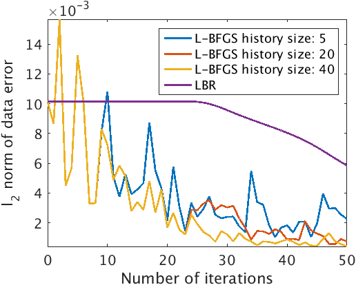
Figure 1 shows the comparison of data error variation with iterations of L-BFGS and Linearized Bregman (LBR) for a given microseismic dataset and for a given value of \(\mu\). We clearly observe that the data error decays faster for LBFGS based method in comparison to Linearized Bregman based method. Here, we choose a higher value of \(\mu\) to get sparse solutions. A higher value of \(\mu\) does not allow the source wavefields \(\vector{Q}\) to be updated in the early iterations. Therefore, the Linearized Bregman algorithm goes through initial phase of stagnation. In Figure 1 we also demonstrate the advantage of storing dual variable updates for improved L-BFGS convergence. We achieve improved convergence without incurring any additional memory cost, since our dual variable lives in data domain. We compare the convergence for update history size of \({5}\), \({20}\) and \({40}\). We observe better convergence with increasing L-BFGS update history size.

Numerical Experiments

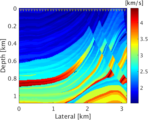
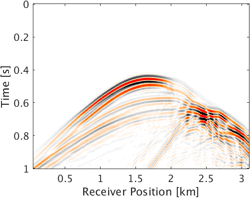
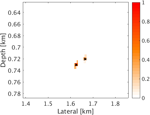
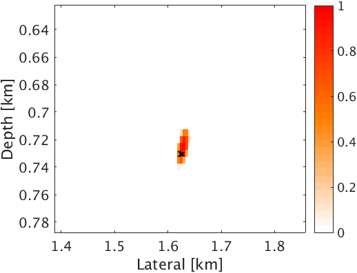
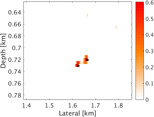
We performed two different experiments to compare the efficacy of the proposed method with respect to Linearized Bregman based method (Sharan et al., 2016). For both of these experiments, we assume that microseismic sources are monopole point sources. To demonstrate the effectiveness of our method in a complex geological situation, we use a part of Marmousi model with dimensions \(3.15\,\mathrm{km} \times 1.08\,\mathrm{km}\) (\(631 \times 217\) points) (Figure 2a). We use \(2.5\)D time-stepping acoustic finite difference modeling code to generate microseismic data. We set surface receivers buried at depth of \(20\,\mathrm{m}\) with separation of \(10\,\mathrm{m}\) to record P-wave data. We use noise free data to simultaneously estimate source location and source time function. For both experiments we consider two closely spaced sources within half a wavelength. The first source is located at (\(1.625\, \mathrm{km}\) , \(0.73\, \mathrm{km}\)) and the second source is located at (\(1.665\, \mathrm{km}\) , \(0.72\, \mathrm{km}\)) (Figure 2a). Both sources are in low velocity zone and separated within half a wavelength. Both sources are activated at different times and with different dominant frequencies of \(30.0\, \mathrm{Hz}\) and \(25.0\, \mathrm{Hz}\) respectively. We use \(1\,\mathrm{s}\) record length of microseismic data (Figure 2b) to jointly estimate the location and source time function of both the sources.

Experiment 1—True velocity experiment

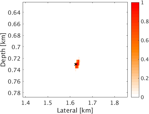
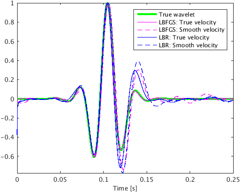
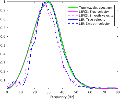
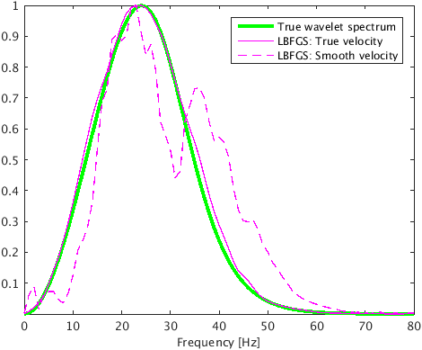
In the first experiment, we assume that we have access to the true velocity model. To compare how proposed method works in comparison to Linearized Bregman algoirthm for our problem, we perform 50 iterations of both the algorithms for same value of \(\mu\). Figure 2c & 2d are intensity plots corresponding to the linearized Bregman and the proposed method based on L-BFGS. The linearized Bregman based method is able to estimate only one source location correctly, namely at (\(1.625\, \mathrm{km}\) , \(0.73\, \mathrm{km}\)) (Figure 2c), whereas the proposed method estimates both source locations correctly after the same number of iterations (Figure 2d). This clearly demonstrates the faster convergence of the proposed method with compared to the linearized Bregman based method. Also, the proposed method is able to give a good estimation of the source time function at both locations, whereas the linearized Bregman based results only recovers one source (Figure 3a & 3b). The proposed method is able to preserve the frequency content of the source time function at both the source locations. This is evident from the amplitude spectrum plot of source time function at both the locations (Figure 3c & 3d). This is because we are working in \(2.5\)D instead of \(2\)D, which prevents any kind of frequency loss due to \(2\)D wave modeling (Z.-M. Song and Williamson, 1995).

Experiment 2—Smooth velocity experiment

In the 2nd experiment we assume that we only have access to a smooth velocity model. We still use the data generated in experiment 1 (Figure 2b), but this time we use a smoothed version of the Marmousi model to jointly estimate the microseismic source location and source time function of both the sources. We use \(125\ \times 125\, \mathrm{m^2}\) \(2\)d filter to smooth the Marmousi model. For same value of \(\mu\) , we perform 100 iterations of linearized Bregman based method and the proposed method to jointly estimate location and source-time function of both the microseismic sources. As before, with the linearized Bregman based method we are able to recover only one source location (Figure 4a) after 100 iterations whereas with the proposed method, we are able to estimate both the source locations (Figure 4b). We get good estimate of the source time function at both the locations with the proposed method, whereas linearized Bregman based method estimates source time function at one source location (Figure 3a). The proposed method also preserves the frequency content of the source time function at both the source locations as evident from the amplitude spectrum plot of source time function at both the locations (Figure 3c & 3d). We observe some noise in the spectrum of estimated source-time function. This is mainly because of the cross-talk between sources within half a wavelength. We can reduce this cross talk by spectral smoothing. With velocity update, we can get further focusing of source field at the true source location, which can further reduce this cross talk. Velocity update is out of scope for this paper but the comparison of results of experiment \(1\) with true velocity and experiment \(2\) with smooth velocity is encouraging.

Conclusions

We have proposed a method to jointly estimate closely spaced microseismic source locations and their source time function functions. Linearized Bregman based method requires lot of iterations for closely spaced sources. However, L-BFGS based method can locate sources within half a wavelength along with their source time function in lesser iterations. The L-BFGS based method works with dual variable which is cheaper to store. Therefore, we can store dual variable updates without any addition memory storage burden to get better L-BFGS convergence. We have extended our method in \(2.5\)D. Lastly, we can estimate location and source time function of more than one sources without any assumptions on number of sources.

Acknowledgement

This research was carried out as part of the SINBAD project with the support of the member organizations of the SINBAD Consortium.