Developments in the direction of solving extremly large problems in Geophysics

Summary

Often in exploration Geophysics we are forced to work with extremely large problems. Acquisitions via dense grids of receivers translate into very large mathematical systems. Usually, depending on the acquisition, the size of the matrix of the system to be solved, can be measured in the millions. The proper way to address this problem is by subsampling. Even though subsampling can reduce the computational efforts required, it can not address stability problems caused by preconditioning and/or instrumental response errors. In this abstract, we introduce a modification of the linearized Bregman solver for these large problems that resolves stability issues.

Introduction

The generalized mathematical formulation in many geophysical applications can be summarized by the following optimization problem: \[ \begin{equation} \min_{x\in\mathbb{R}^n} F(x)\;\;\;\; s.t.\;\;\;\;\; Ax=b, \label{BP} \end{equation} \] where \(F(x)\) is a convex function, \(A\) represents a modeling operator, and \(b\) is the acquisition data, organized in a very specific way. The problem ( \(\ref{BP}\) ) becomes extremely large and eventually we have to subsample (Lorenz et al., 2014 , Herrmann et al. (2015)) in order to make the problem computationally feasible.

Reducing the computational cost is very important and desired. A very fast, simple and efficient method for the the problem ( \(\ref{BP}\) ) is the linearized Bregman (Lorenz et al., 2014 ), which is described as : \[ \begin{equation} \begin{aligned} \begin{array}{lcl} z_{k+1} & = & z_k-t_k A_k^T(A_k x_{k}-b_k)\\ x_{k+1} & = & S_{\lambda}(z_{k+1}), \end{array} \end{aligned} \label{LB} \end{equation} \] where \(S_{\lambda}(z_{k+1})=sign(z_{k+1})\max \{0, |z_{k+1}|-\lambda \}\), \(t_k=\frac{||A_k x_k-b||_2^2}{||A_k^T(A_k x_k-b)||_2^2}\) called the “dynamic time-step”, the index \(k\) denotes a subsampling of the operator \(A\) and \(b\) is the data. The convergence of linearized Bregman is proven in the case where \(Ax=b\), corresponding to \(\ref{BP}\) as a consistent problem.

In practice, since the data are subject to several preprocessing steps, it is typical that \(b=Ax+w\), where \(w\) is the effect of the preprocessing. This makes the problem inconsistent and it is not guaranteed that the linearized Bregman method will converge to the exact solution. More precisely the linearized Bregman method will exhibit unstable behavior, no longer converging to an exact solution but instead alternating between (approximate) feasible solutions. In Figure 1 we demonstrate this unstable behavior by following a single entry of the linearized Bregman solution of a toy problem. We observe that the solution of the Bregman method, after iteration 8, cycles around the exact value for the \(Ax=b\) and stops converging to a single solution.

In this abstract we show that the intensity of this cycling behaviour increases with the size of the system. We have associated the intensity of this behavior with the dynamic time step \(t_k\) used for improving the convergence rate in the linearized Bregman method. We propose a weighted increment, which allows the linearized Bregman to converge to a feasible solution.

We provide an example of LS migration problems that translates into an optimization problem of the form ( \(\ref{BP}\) ) . We discuss the advantages of the proposed modification of the linearized Bregman method.

Linearized Bregman with weighted increment

Solving a highly overdetermined, inconsistent system with linearized Bregman, introduces many challenges as demonstrated in Figure 1 . These challenges are driven by the combination of the form of the dynamic time step \(t_k\) in the method and from the tendency of the linearized Bregman method to overfit the noise in the data. Further contributing to these difficulties, in LS migration problems (Herrmann et al., 2008 ) we have to invert a highly overdetermined problem and the inconsistency comes from several preprocessing step for the data.

To avoid overfitting the noise, we propose a small but very effective modification of the linearized Bregman algorithm : \[ \begin{equation} \begin{aligned} \begin{array}{lcl} z_{k+1} & = & z_k-\tau_k \odot A_k^T(A_k x_{k}-b_k)\\ x_{k+1} & = & S_{\lambda}(z_{k+1}), \end{array} \end{aligned} \label{LB2} \end{equation} \] where \(\odot\) denotes element wise multiplication. We introduce a weight factor in the incrementand given by \[ \begin{equation} \tau_k^i=t_k \dfrac{|\sum\limits_{j=1}^{k}\operatorname{sign}\big([A_j^T(A_j x_j-b_j)]_i\big)|}{k}. \label{weights} \end{equation} \] The increment of the linearized Bregman in ( \(\ref{LB2}\) ) allows us to adapt the increment independently for every entry of the solution vector and we can reduce the increment to values close to zero whenever an entry is close to the desired value. The weighted increment can drastically reduce the model error of the method.

A RELATED CHALLENGE IN GEOPHYSICS

The LS migration problem ( \(\ref{CS}\) ) translates into an inverse problem equivalent to the problem ( \(\ref{BP}\) ). \[ \begin{equation} \min_{x} ||x||_1\;\;\;\;\text{s.t.}\;\;\;\sum\limits_{i=1}^{n_s}||\mathbf{J}_i[\mathbf{m}_0,\mathbf{q}_i]\mathbf{C}^*x-\mathbf{b}_i||_2\leq\sigma. \label{CS} \end{equation} \] Here \(x\) is a vector of the Curvelet coefficients, \(\mathbf{J}_i\) is the Born modelling operator for the \(i^{th}\) shot, \(\mathbf{m}_0\) is the background model for the velocity, \(\mathbf{q}_i\) is the source wavelet for the \(i^{th}\) shot, \(\mathbf{b}_i\) is the vectorized reflection for \(i^{th}\) shot, \(\mathbf{C}^*\) is the transpose of the Curvelet transform and \(\sigma\) is the noise tolerance or modeling error.

The role of the matrix \(A\) in the problem \(\ref{BP}\) is performed by the operator \(\mathbf{J}_i[\mathbf{m}_0,\mathbf{q}_i]\mathbf{C}^*\). The Curvelet coefficients of the vector \(x\) decay exponentially, meaning that just a few coefficients have large value and the vast majority of them are very small. This makes the vector \(x\) compressible.

The effectiveness of the weighted increment

The effectiveness of the proposed weighted increment is demonstrated by the following experiment. To keep the experiment closely related to the LS migration problem, the objective is to recover a vector of Curvelet coefficients. The matrix \(A\) is a tall \(10000000\times 2040739\) operator, which will replace the corresponding modelling operator of the LS migration problem. The data is generated by applying a known operator \(A\) to a known vector of Curvelet coefficients. Finally, to simulate the inconsistency of the problem, we add noise to the data.

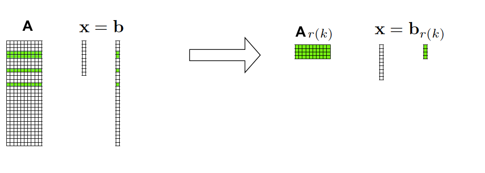
We solve ( \(\ref{BP}\) ) using the linearized Bregman method and then again using the proposed modification using the weighted increment. In every iteration we are solving an underdetermined problem by using a submatrix \(A_k\), which contains 500000 randomly selected rows of \(A\) as illustrated by the schematic of Figure 2 .

In Figure 3 we show the relative model error for the first 150 iterations for both methods. The model error of the linearized Bregman stagnates at about \(5\%\), while the model error using the weighted increment method drops to about \(3\%\) and continues to decrease with more iterations..

The error difference between the original linearized Bregman and the modified method using the weighted increment is related to the unstable behaviour with cycling that we demonstrated in Figure 1 . It is this cycling behavior in the standard linearized Bregman method that is directly responsible for the stagnation of the model error at a large value.

CHALLENGES IN LARGE SCALE PROBLEMS

The explorational Geophysic community is forced by the nature of their problems to implement any specific methodology on a large scale (from 2D to 3D or extented acquisitions, etc). However solving an optimization problem, such as the problem \(\ref{BP}\), becomes exceptionally challenging in large scale. As already demonstrated above, the original linearized Bregman model given in ( \(\ref{LB}\) ) , fails to converge to a feasible solution. Within a large scale problem, this difficulty is magnified, since the increased computational costs usually implies fewer passes through the data, or a smaller number of iterations.

We replicate a large scale problem, by recovering a known Curvelet coefficient vector, with \(A\) to be a \(100000000\times 2040739\), taking the SNR for the large scale problem to be the same as the small scale problem. The configuration of the linearized Bregman method remains the same as the small scale problem so the only difference is the scale.

In Figure 4 we see that the relative model error for the original linearized Bregman method stagnates again, this time at about \(14\%\). The proposed weighted increment linearized Bregman method is performing much better, since the error does not stagnate and continues to decrease throughout th 150 iterations.

For the original linearized Bregman method, the model error stagnates at different levels for the small and the large scale problems. The SNR of the data is the same for both problems, but the size of the data vector is 10 times bigger for the large scale problem. This essentially means that the \(\ell_2\)-norm of the residual is much bigger for the large scale problem. The \(\ell_2\)-norm of the residual is a controlling factor for the unstable cycling behavior demonstrated in Figure 1 and thus the difference in the stagnation level.

As we solve larger and larger problems, the stagnation at a larger model error limits the size of the problem for which a solution can be recovered with acceptable error.

We can remove this limitation with the proposed weighted time-step of equation \(\ref{weights}\) . Using the weighted increment we are only limited by the number of iterations we can afford to do.

Applications in Geophysics and future work

We already have implemented the proposed weighted time-step for 2D least-square migration problems with the result showing how it provides significant improvements in the model error, relative to the original linearized Bregman (see Figure 5 ). While the results so far are impressive, the most promising aspect of the proposed methodology is the stability which is conserved for large scale problems.

Future work includes the impementation of 3D LS migration in time domain. In future work we also include LS migration using ambient noise data instead of shot gathers.

Conclusions

The linearized Bregman solver for inconsistent problems lacks stability, failing to converge to a feasible solution. Furthermore, the overwhelming size of the large scale problems produces additional errors. In this abstract we propose a relatively simple modification to the linearized Bregman solver, which allows us to resolve these problems and preserve the results for large scale problems.

Acknowledgement

This research was carried out as part of the SINBAD project with the support of the member organizations of the SINBAD Consortium. Partially supported by a Natural Sciences and Engineering Research Council Accelerator Grant.