Reconstruction of S-waves from low-cost randomized and simultaneous acquisition by joint sparse inversion

Ali M. Alfaraj*, Rajiv Kumar and Felix J. Herrmann
Seismic Laboratory for Imaging and Modelling (SLIM), University of British Columbia

Introduction

Multicomponent ocean bottom seismic data carries valuable shear (S-wave) information that enables numerous applications such as imaging through a gas cloud and high resolution shallow subsurface imaging (Stewart et al., 2003). In order to obtain pure up- and down-going compressional (P-waves) and S-waves from recorded multicomponent data, we need to perform elastic wavefield decomposition just below the ocean bottom (C.P.A. Wapenaar and Berkhout, 2014). However, the velocity of the S-waves are much slower than that of with P-waves, which makes the earlier aliased when recorded with conventional acquisition designs targeted towards acoustic imaging. To avoid aliasing by satisfying the Nyquist sampling criterion, which requires the spatial sampling to be proportional to the apparent subsurface velocity, and to use the multicomponent data to its full available extent, denser source and/or receiver sampling is required. This leads to prohibitively high acquisition costs, which limits the use of S-waves. On the other hand, we can avoid aliasing of the S-waves without increasing the acquisition costs by utilizing ideas from the field of compressive sensing (Donoho, 2006; Candès and Wakin, 2008; Hennenfent and Herrmann, 2008). Instead of dense sampling, we propose acquiring data in a randomly undersampled fashion. The data can then be interpolated from a coarse grid into a uniform fine grid. There exist different interpolation methods that use the properties of various transforms. These include the Fourier transform (Zwartjes and Sacchi, 2007), curvelet transform (Hennenfent and Herrmann, 2006, 2008), Radon transform (Trad et al., 2002, Kabir and Verschuur (1995)), and frequency-wavenumber transform (Stanton and Sacchi, 2013). In our recent publication (Alfaraj et al., 2017), we have interpolated each component of randomly subsampled multicomponent ocean bottom seismic data independently and then decomposed the interpolated components into up- and down-going S-waves. In this work, we move from a two-step to a one-step approach so that we can handle all the multicomponent data in one optimization scheme and preserve their relative amplitudes. We jointly interpolate and decompose the multicomponent data by solving one sparsity-promoting optimization problem where the input is the randomly subsampled multicomponent data and the desired outputs are the densely sampled up- and down-going S-waves. We formulate the problem using sparsity promotion in two domains: the curvelet domain and the frequency-wavenumber domain. Another important acquisition key factor is the overall acquisition time. By acquiring seismic data with simultaneous sources, larger areas can be covered in shorter acquisition times (Beasley, 2008). Wason and Herrmann (2013) have shown that data can be deblended with sparsity promotion in the curvelet domain. Since our final goal is to reconstruct up- and down-going S-waves, we implement the source separation and decomposition in a one-step approach by solving a sparsity promoting joint source separation decomposition.

This paper is organized as follows. We first explain the theory of elastic wavefield decomposition and wavefield composition, followed by explanation of the theory of sparsity promoting joint interpolation decomposition and joint source separation decomposition. Next we demonstrate our proposed schemes on synthetic elastic finite-difference data.

Elastic wavefield decomposition

The measured multicomponent two-way wavefields \(\mathbf{q}\) can be decomposed into one-way wavefields \(\mathbf{d}\) using a decomposition matrix \(\mathbf{N}\) in the frequency-wavenumber (f-k) domain as follows: \[ \begin{equation} \mathbf{d} = \mathbf{N}\mathbf{q}. \label{eq:elD-1} \end{equation} \] The two-way wavefields can also be composed from one-way wavefields using a composition matrix \(\mathbf{L}\): \[ \begin{equation} \mathbf{q} = \mathbf{L}\mathbf{d}. \label{eq:elQ-1} \end{equation} \] For the elastic case, the one-way wavefields contain the P-wave potential \(\mathbf{\phi}\) and the S-wave potential \(\mathbf{\psi}\), while the two-way wavefields contain the traction \(\mathbf{\tau}\) and the particle velocity \(\mathbf{v}\). We consider waves polarized in the horizontal-vertical (\(x-z\)) plane, neglect SH waves and only consider P-SV waves. The decomposed potentials in the f-k domain for two-dimensional media can be obtained by (C.P.A. Wapenaar and Berkhout, 2014; CPA Wapenaar et al., 1990): \[ \begin{equation} \begin{aligned} \left(\begin{array}{c} \phi^+\\ \psi_y^+\\ \phi^-\\ \psi_y^- \end{array}\right) = \left(\begin{array}{cc} \mathbf{N}_{1}^+ & \mathbf{N}_{2}^+ \\ \mathbf{N}_{1}^- & \mathbf{N}_{2}^- \end{array}\right) \left(\begin{array}{c} -\tau_{xz}\\ -\tau_{zz}\\ v_{x}\\ v_z \end{array} \right). \end{aligned} \label{eq:D} \end{equation} \] We can obtain the composed two-way wavefields by: \[ \begin{equation} \begin{aligned} \left(\begin{array}{c} -\tau_{xz}\\ -\tau_{zz}\\ v_{x}\\ v_z \end{array} \right) = \left(\begin{array}{cc} \mathbf{L}_{1}^+ & \mathbf{L}_{1}^- \\ \mathbf{L}_{2}^+ & \mathbf{L}_{2}^- \end{array}\right) \left(\begin{array}{c} \phi^+\\ \psi_y^+\\ \phi^-\\ \psi_y^- \end{array}\right), \end{aligned} \label{eq:Q} \end{equation} \] where \(\tau_{xz}\) and \(\tau_{zz}\) represent the shear and normal tractions, \(v_{x}\) and \(v_{z}\) are the horizontal and vertical particle velocity components, the superscripts \(^-\) and \(^+ \) indicate up- and down-going wavefields, respectively. At the ocean bottom, the shear traction vanishes, while the normal traction equals the negative of the acoustic pressure, (Aki and Richards, 2002). We assume we know the ocean floor properties required for composing and decomposing the wavefields. Schalkwijk et al. (2003) showed that these properties can be be estimated with an adaptive wavefield decomposition scheme while Alfaraj et al. (2015) showed that they can be estimated with wavefield tomography. From alias-free measurements at the ocean bottom, we can now obtain the up- and down-going P- and S-waves. We can also obtain the two-way wavefields by composing the up- and down-going one-way wavefields. However, when the multicomponent data is acquired with not fine enough spatial sampling, the S-waves become aliased and impractical to use.

Joint-interpolation decomposition

The Nyquist sampling criterion imposes prohibitively high acquisition costs when acquiring finely sampled multicomponent data specifically targeted towards S-waves. In order to be able to use the valuable information the S-waves have to offer without increasing the acquisition costs, we utilize ideas from the field of compressive sensing by placing sources and/or receivers on a randomly subsampled grid. With such sampling, aliasing is turned into incoherent noise in a transform domain which enables us to formulate the interpolation problem as a denoising problem (Hennenfent and Herrmann, 2006, 2008; Herrmann et al., 2012). Given randomly subsampled multicomponent data (\(\mathbf{p}, \mathbf{v}_z, \mathbf{v}_x\)) represented by \(\mathbf{b} \in \mathbb{R}^n\), we wish to reconstruct the fully sampled up- and down-going P- and S-waves represented by \(\mathbf{f} \in \mathbb{R}^N\), where \(n \ll N\). We assume that the data has a sparse representation \(\mathbf{x} \in \mathbb{C}^P\) given by the transform operator \(\mathbf{S} \in \mathbb{C}^{P \times N} \), where \(P \geq N\). The subsampled multicomponent data \(\mathbf{b}\) is related to the transform domain coefficients \(\mathbf{x}\) and the reconstructed data \(\mathbf{f}\) by the matrix \(\mathbf{A} \in \mathbb{C}^{n \times P}\), and the subsampling matrix \(\mathbf{R} \in \mathbb{R}^{n \times P}\), respectively: \[ \begin{equation} \mathbf{A}\mathbf{x} = \mathbf{R}\mathbf{f} = \mathbf{b}. \label{eq:Axb} \end{equation} \] When using the frequency-wavenumber transform as the sparsifying transform, \(\mathbf{A}\) is defined as follows: \[ \begin{equation} \mathbf{A}_{fk} = \mathbf{R} \mathbf{F}^H \mathbf{L}, \label{eq:Afk} \end{equation} \] where \(\mathbf{L} \in \mathbb{C}^{P \times P}\) is the composition operator, \(\mathbf{F} \in \mathbb{C}^{P \times P}\) is the 2D Fourier transform and the superscript \(^H\) denotes the Hermitian transpose. When using the curvelet transform as the sparsifying transform, \(\mathbf{A}\) becomes: \[ \begin{equation} \mathbf{A}_c = \mathbf{R} \mathbf{F}^H \mathbf{L} \mathbf{F} \mathbf{C}^H, \label{eq:Ac} \end{equation} \] where \(\mathbf{C} \in \mathbb{C}^{P \times N}\) is the curvelet transform operator. To reconstruct the up- and down-going P- and S-waves directly, we solve the following convex optimization problem: \[ \begin{equation} \min_{\mathbf{x} \in \mathbb{C}^P} \|\mathbf{x}\|_1 \quad\text{subject to } \quad \| \mathbf{A} \mathbf{x} - \mathbf{b}\|_2 \leq \sigma \label{eq:BPDN} \end{equation} \] using the SPG\(\ell_1\) solver (Berg and Friedlander, 2008). The parameter \(\sigma\) is the noise level and \(\|\mathbf{x}\|_1\) is the sum of the absolute values of the elements of \(\mathbf{x}\). Since we input all the subsampled multicomponent data in one optimization problem, we benefit from not having to solve and tune separate optimizations problem for each component. When interpolating each component separately, the outcome may not honor the relative amplitude values between the components. Therefore, amplitudes of each component as well as the noise effect have to be studied carefully before and after reconstruction. While in the joint-interpolation decomposition case, the information from each component is weighted by multiplication with appropriate factors in the composition operator, which ensures having correct decomposition results.

Joint-source separation decomposition

Simultaneous source acquisition aims at reducing the acquisition time by covering larger areas in shorter times. Instead of separately deblending each component of the data and then retrieving the up- and down-going P- and S-waves, we propose performing these two steps jointly by solving a sparsity promoting joint source separation decomposition problem. We follow the same approach as in the previous section, but rather than randomly subsampling the data, we apply a Gaussian independent and identically distributed (i.i.d.) random matrix to each component of the data to mitigate a blended acquisition scenario. We should note that this measurement matrix is more appropriate for land acquisition where we can have multiple vibrators firing at random times with different phase encodings, which is not feasible for marine acquisition up to now. We solve the same basis of pursuit denoising problem, equation \(\ref{eq:BPDN}\), where our observed data \(\mathbf{b}\) becomes the simultaneously acquired multicomponent data and our outputs of interest are the deblended up- and down-going S-waves.

Numerical results and discussion

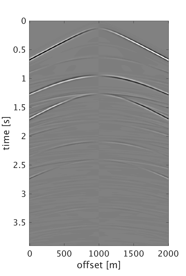
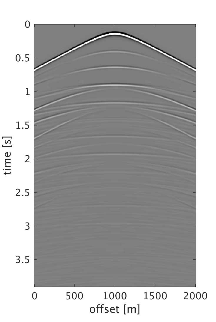
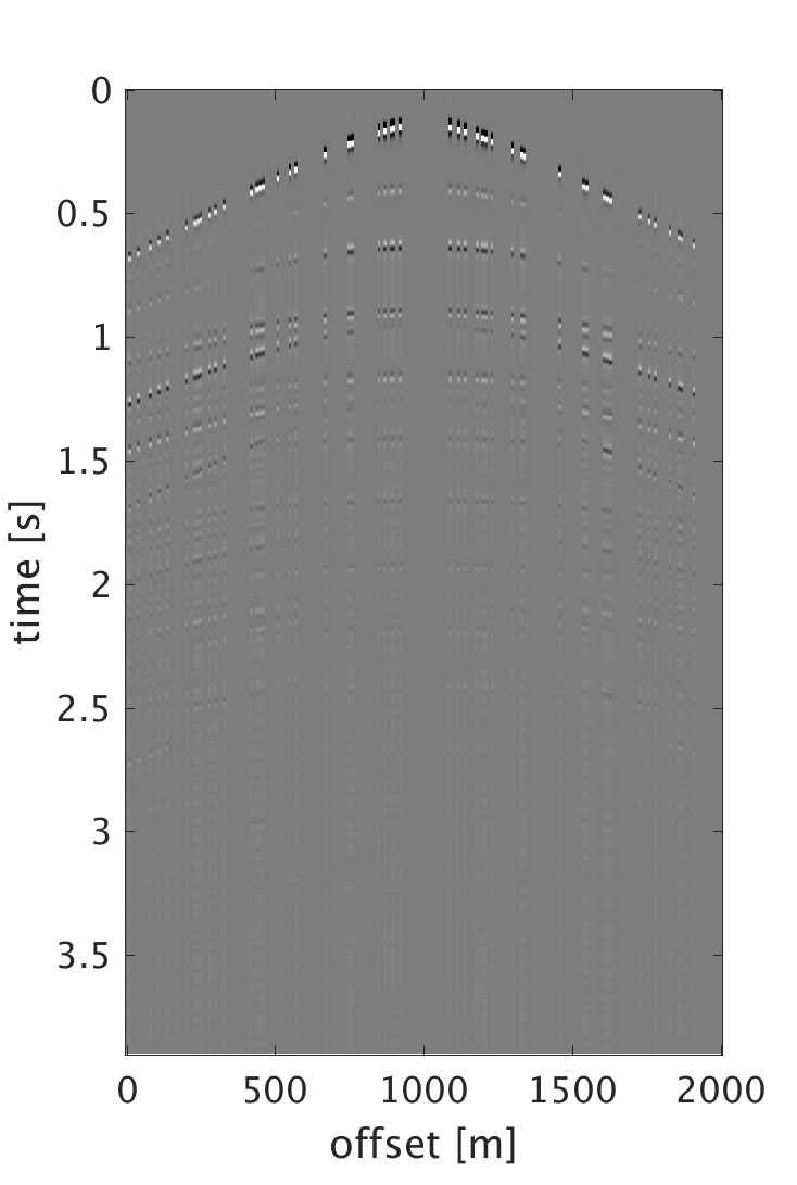
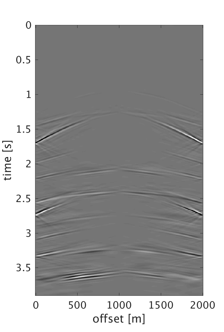
We demonstrate the performance of our proposed schemes on 200 shots and 200 multicomponent receivers modeled using a 2D elastic finite-difference modeling code (Thorbecke and Draganov, 2011), figure 1. The source and receiver intervals are 10 m and the maximum frequency of the data is 60 Hz. Figure 3 shows the decomposition results of the dense data. We randomly subsample each component by removing 75% of the data, where the largest and smallest gaps are 200 m and 10 m respectively, figure 2. We then perform sparsity promoting joint interpolation decomposition to directly reconstruct the up- and down-going P- and S-waves, figure 4. The results obtained by using \(\mathbf{A}_c\) that corresponds to the curvelet domain are much better compared with the results obtained with \(\mathbf{A}_{fk}\), which corresponds to the frequency-wavenumber domain. The latter has more noise, which we attribute to the fact that curvelet coefficients are capable of capturing the variations of seismic data and providing a sparser representation than the frequency-wavenumber coefficients. Even though the formulation of \(\mathbf{A}_c\) seems computationally expensive, it only requires 20 iterations to converge to the results. Since the composition operator is applied in the frequency-wavenumber domain, we have also studied the performance of the algorithm when we change \(\mathbf{A}_c\) to \[ \begin{equation} \mathbf{A}_{c2} = \mathbf{L} \mathbf{F} \mathbf{R} \mathbf{C}^H, \label{eq:Ac_fk} \end{equation} \] and formulate our observed data \(\mathbf{b}\) to be in the frequency-wavenumber domain. This reduces the computation cost since we end up with only one frequency-wavenumber transform in \(\mathbf{A}_{c2}\). However, the results get degraded since we are applying the subsampling operator directly on the one-way decomposed data, which in reality is not the case. What is being subsampled in the field are the multicomponent measurements. Therefore using the subsampled decomposed wavefields to form the two-way wavefields results in artifacts that distorts the quality of the recovery. For the simultaneous sources experiment, we implement the sparsity-promoting joint source separation interpolation on the fully sampled dataset to recover the up- and down-going S-waves, figure 5. We observe similar results to the joint interpolation decomposition where the curvelet domain formulation performs better than the frequency wave-number domain formulation.

We have demonstrated that we are able to recover reasonably accurate up- and down-going S-waves from (i) 75% randomly missing multicomponent data and from (ii) simultaneously acquired data by performing sparsity-promoting joint-interpolation decomposition and joint-source separation decomposition, respectively. As a result, we move away from performing each step independently, which leads to several benefits. We end up with an algorithm that can handle all the multicomponent data in one go, not only to interpolate or deblend the data, but also to provide up- and down-going P- and S-waves. This leads to having less tuning parameters of the optimization problem as well as less overall computation time. Moreover, the relative amplitude values amongst the components get preserved, which should in principle lead to better decomposition results. This makes the joint formulations more favorable than the multi-step formulations. Future work should include examining the noise effect and performing P-S migration of the decomposed data.

Conclusions

S-waves are slower than P-waves, which makes them either aliased or more expensive when acquired with conventional acquisition designs as they require much finer spatial sampling. We propose acquiring the S-waves by randomized undersampling, which is a more economical way of acquiring the data. Aliased energy is then turned into incoherent noise in the sparse domain. This allows using the sparsity promotion advantages to perform joint-interpolation decomposition where we solve for the up- and down-going S-waves directly from randomly subsampled multicomponent data. To reduce the acquisition time and efficiently acquire seismic data, simultaneous source acquisition is becoming the standard of collecting seismic data. This requires a deblending step. Instead of taking a two-step approach by deblending then decomposing, we jointly deblend and decompose the multicomponent data into up- and down-going P- and S-waves. When performing the proposed joint schemes, we are more confident that the relative amplitudes of the multicomponent data are preserved. Synthetic data results show that by implementing the sparsity promoting joint source separation decomposition and joint interpolation decomposition, we are able recover reasonably accurate up- and down-going S-waves.

Acknowledgements

Ali Alfaraj extends his gratitude to Saudi Aramco for sponsoring his Ph.D. studies at the University of British Columbia. This research was carried out as part of the SINBAD project with the support of the member organizations of the SINBAD Consortium.