Time-domain sparsity-promoting least-squares migration with source estimation

Summary:

Traditional reverse-time migration (RTM) gives images with wrong amplitudes and low resolution. Least-squares RTM (LS-RTM) on the other hand, is capable of obtaining true-amplitude images as solutions of \(\ell_2\)-norm minimization problems by fitting the synthetic and observed reflection data. The shortcoming of this approach is that solutions of these \(\ell_2\) problems are typically smoothed, tend to be overfitted, and computationally too expensive because it requires compared to standard RTM too many iterations. By working with randomized subsets of data only, the computational costs of LS-RTM can be brought down to an acceptable level while producing artifact-free high-resolution images without overfitting the data. While initial results of these “compressive imaging” methods were encouraging various open issues remain including guaranteed convergence, algorithmic complexity of the solver, and lack of on-the-fly source estimation for LS-RTMs with wave-equation solvers based on time-stepping. By including on-the-fly source-time function estimation into the method of Linearized Bregman (LB), on which we reported before, we tackle all these issues resulting in a easy-to-implement algorithm that offers flexibility in the trade-off between the number of iterations and the number of wave-equation solves per iteration for a fixed total number of wave-equation solves. Application of our algorithm on a 2D synthetic shows that we are able to obtain high-resolution images, including accurate estimates of the wavelet, for a single pass through the data. The produced image, which is by virtue of the inversion deconvolved with respect to the wavelet, is roughly of the same quality as the image obtained given the correct source function.

Introduction

Reverse-time migration (RTM) approximates the inverse of the linearized Born modelling operator by its adjoint. As a consequence, RTM without extensive preconditioning—generally in the form of image domain scalings and source deconvolution prior to imaging—cannot produce high-resolution true-amplitude images. By fitting the observed reflection data in the least-squares sense, least-squares migration, and in particular least-squares reverse-time migration (LS-RTM), overcomes these issues except for two main drawbacks withstanding their succesful application. Firstly, the computational cost of conducting demigrations and migrations iteratively is very large. Secondly, minimizing the \(\ell_2\) norm of the data residual can lead to model perturbations with artifacts caused by overfitting. These are due to the fact that LS-RTM involves the inversion of a highly overdetermined system of equations where it is easy to overfit noise in the data.

One approach to avoid overfitting is to apply regularization to the original formulation of LS-RTM, and search for the sparsest possible solution by minimizing the \(\ell_1\)-norm on some sparsifying representation of the image. Motivated by the theory of Compressive Sensing (Donoho, 2006), where sparse signals are recovered from severe undersamplings, and considering the huge cost of LS-RTM we turn the overdetermined imaging problem into a underdetermined one by working with small subsets of sources at each iteration of LS-RTM, reducing the computational costs.

Herrmann et al. (2008) found that, as a directional frame expansion, curvelets lead to sparsity of seismic images in imaging problems. This property led to the initial formulation of curvelet-based “Compressive Imaging” (Herrmann and Li, 2012), which formed the bases of later work by Tu et al. (2013) who included surface-related multiples and on-the-fly source estimation via variable projection. While this approach represents major progress the proposed method, which involves drawing new independent subsets of shots after solving each one-norm constrained subproblem, fails to continue to bring down the residual. This results in remaining subsampling related artifacts. In addition, the proposed method relies on a difficult to implement one-norm solver. To overcome these challenges, F. J. Herrmann et al. (2015) motivated by Lorenz et al. (2014) relaxed the one-norm objective of Basis Pursuit Denoise (Chen et al., 2001) by an objective given by the sum of the \(\lambda\)-weighted \(\ell_1\)- and \(\ell_2\)-norms. This seemingly innocent change resulted in a greatly simplified implementation that no longer relies on relaxing the one-norm constraint and more importantly provably continues to make progress towards the solution irrespective of the number of randomly selected sources participating in each iteration.

Inspired by this work, we propose to extend our earlier work in frequency domain to the time domain, which is more appropriate for large scale 3D problems and to include on-the-fly source estimation via variable projection. Both generalizations are completely new and challenging because the estimation of the time-signature of the source wavelet no longer involves estimating a single complex number for each temporal frequency (Tu et al., 2013).

Our paper is organized as follows. First, we formulate sparsity-promoting LS-RTM as a Basis Pursuit Denoising problem formulated in the curvelet domain. Next, we relax the \(\ell_1\)-norm and describe the relative simple iterative algorithm that solves this optimization with the mixed \(\ell_1\)- \(\ell_2\)-norm objective. We conclude this theory section by including estimation of the source-time signature that calls for additional regularization prevent overfitting of the wavelet. We evaluate the performance of the proposed method on the synthetic SIGSBEE2A model (Paffenholz et al., 2002) where we compare our inversion results to LS-RTM with the true source function and standard RTM.

Theory

Imaging with linearized Bregman

The original sparsity-promoting LS-RTM has the same form, albeit it is overdetermined rather than underdetermined, as Basis Pursuit Denoise (BPDN, Chen et al. (2001)), which is expressed as below \[ \begin{equation} \begin{aligned} & \min_{\vector{x}} \ \Vert \vector{x} \Vert_1 \\ & \text{subject to} \quad \sum_{i} \Vert \nabla \vector{F}_{i}( \vector{m}_0, q_i) \vector{C}^T \vector{x} - \delta \vector{d}_{i}\Vert \leq \sigma, \end{aligned} \label{BP} \end{equation} \] where the vector \(\vector{x}\) contains the sparse curvelet coefficients of the unknown model perturbation. The symbols \(\Vert \cdot \Vert_1\) and \(\Vert \cdot \Vert\) denote \(\ell_1\) and \(\ell_2\) norms, respectively. The matrix \(\vector{C}^T\) is the transpose of curvelet transform \(\vector{C}\). The vectors \(\vector{m}_0\) stands for the background velocity model and \(q_i=q_i(t)\) is the time dependent source function for the \(i^{th}\) shot. The matrix \(\nabla\vector{F}_{i}\) and vector \(\delta \vector{d}_{i}\) represent the linearized Born modelling operator and observed reflection data along the receivers for the \(i^{th}\) shot. The \(\sum_{i}\) runs over all shots. The parameter \(\sigma\) is the noise level of the data.

Despite the success of BPDN in Compressive Sensing, where matrix-vector multiplies are generally cheap, solving Equation \(\ref{BP}\) in the seismic setting where the evaluation of the \(\nabla\vector{F}_{i}\)’s involve wave-equation solves is a major challenge because it is computationally infeasible. To overcome this computational challenge, Herrmann and Li (2012) proposed, motivated by ideas from stochastic gradients, to select subsets of shots by replacing the sum over \(i=1\cdots n_s\), with \(n_s\) the number of shots, to a sum over randomly selected index sets \(\mathcal{I}\in [1 \cdots n_s]\) of size \(n^{\prime}_{s}\ll n_s\). By redrawing these subsets at certain points of the \(\ell_1\)-norm minimization, Li et al. (2012) and Tu et al. (2013) were able to greatly reduce the computational costs but at the expense of giving up convergence when the residual becomes small.

For underdetermined problems, Cai et al. (2009) presented a theoretical analysis that proves convergence of a slightly modified problem for iterations that involve arbitrary subsets of rows (= subsets \(\mathcal{I}\)). F. J. Herrmann et al. (2015) adapted this idea to the seismic problem and early results suggest that the work of Cai et al. (2009) can be extended to the overdetermined (seismic) case. With this assumption, we propose to replace the optimization problem in Equation \(\ref{BP}\) by \[ \begin{equation} \begin{aligned} \min_{\vector{x}} \ & \lambda \Vert\vector{x} \Vert_1 + \frac{1}{2} \Vert\vector{x} \Vert^2 \\ & \text{subject to} \ \sum_{i} \Vert \nabla \vector{F}_{i}( \vector{m}_0, q_i) \vector{C}^T \vector{x} - \delta \vector{d}_{i}\Vert \leq \sigma. \end{aligned} \label{PlainLB} \end{equation} \] Mixed objectives of the above type are known as elastic nets in machine learning and for \(\lambda\rightarrow\infty\)—which in practice means \(\lambda\) large enough—solutions of these modified problems converge to the solution of Equation \(\ref{BP}\). While adding the \(\ell_2\)-term may seem an innocent change, it completely changes the iterations of sparsity-promoting algorithms including the role of thresholding (See F. J. Herrmann et al. (2015) for more discussion).

Pseudo code illustrating the iterations to solve Equation \(\ref{PlainLB}\) are summarized in Algorithm 1.

In Algorithm 1, \(t_k = \Vert \vector{A}_k \vector{x}_k - \vector{b}_k\Vert^2 / \Vert \vector{A}_k^T (\vector{A}_k \vector{x}_k - \vector{b}_k)\Vert^2\) is the dynamic stepsize and \(S_{\lambda}(\vector{z})\) is the soft thresholding operator (Lorenz et al., 2014), and \(\mathcal{P}_\sigma\) projects the residual onto a \(\ell_2\)-norm ball given by the size of the noise \(\sigma\). To avoid too many iterations, the threshold \(\lambda\), which has nothing to do with the noise level but with the relative importance of the \(\ell_1\) and \(\ell_2\)-norm objectives, should be small enough, usually set proportional to the level of the maximum of \(\vector{z}_k\) to let entries of \(\vector{z}_k\) enter into the solution.

On-the-fly source estimation

Algorithm \(\ref{BP}\) requires knowledge of the source-time signatures \(q_i\) to be successfully employed. Unfortunately, this information is typically not available. Following our earlier work on source estimation in time-harmonic imaging and full-waveform inversion (Tu and Herrmann, 2015; Leeuwen et al., 2011), we propose an approach where after each model update, we estimate the source-time function by solving a least-squares problem that matches predicted and observed data.

For the source estimation, we assume that we have some initial guess \(q_0=q_0(t)\) for the source, which convolved with a filter \(w=w(t)\) gives the true source function \(q\). \[ \begin{equation} \begin{aligned} \min_{\vector{x}} \ & \lambda \Vert\vector{ x} \Vert_1 + \frac{1}{2} \Vert \vector{x} \Vert^2 \\ & \text{subject to} \ \sum_{i} \Vert \nabla \vector{F}_{i}( \vector{m}_0, w \ast q_0 ) \mathbf{C}^T \vector{x} - \delta \vector{d}_{i}\Vert \leq \sigma, \end{aligned} \label{LBwithW} \end{equation} \] where \(\ast\) stands for convolution along time. The filter \(w\) is unknown, and needs to be estimated in every Bregman step by solving an additional least-squares subproblem. Generally, estimating \(w\) requires numerous recomputations of the linearized data. This can be avoided by assuming that the linearized data for the current estimated of \(w\) is given by modelling the data with the initial source \(q_0\) and convolving with the filter \(w\) afterwards: \(\nabla\vector{F}_{i}(\vector{m}_0, w \ast q_0) \approx w \ast \nabla\vector{F}_{i}(\vector{m}_0, q_0)\), where the right hand side stands for trace by trace convolution of \(w\) with the shot gather traces.

We expect the estimated source signature to decay smoothly to zero with few oscillations within a short duration of time. Therefore in our subproblem, we add a penalty term \(\Vert r (w \ast q_0) \Vert^2\), where \(r\) is a weight function that penalizes non-zeros entries at later times. In our example we choose \(r\) to be a logistic loss function (Rosasco et al., 2004) as below. Furthermore we add a second penalty term \(\lambda_2 \Vert w \ast q_0 \Vert^2\) to control the overall energy of the estimated wavelet. Our subproblem for source estimation is then given by \[ \begin{equation} \begin{aligned} \min_{w} \ & \sum_i \Vert w \ast \nabla\vector{F}_{i}(\vector{m}_0, q_0) - \delta \vector{d}_i\Vert ^2 \\ & + \Vert r (w \ast q_0) \Vert^2 + \lambda_2 \Vert w \ast q_0 \Vert^2 . \end{aligned} \label{sub22} \end{equation} \] and the weight function \(r\) is defined as

\[ \begin{equation} \begin{aligned} r= \begin{cases} \log (1+e^{\alpha (t-t_0)}) & \mathsf{if} \ t \leq t_0 \\ t-\log (1+e^{\alpha (t_0 -t)}) & \mathsf{if} \ t > t_0 . \end{cases} \end{aligned} \label{Weight} \end{equation} \]

The algorithm to solve the sparsity-promoting LS-RTM with source estimation using linearized Bregman is summarized in Algorithm 2.

In Algorithm 2, \(\star\) stands for correlation, which is the adjoint operation of convolution. Since the initial guess of \(\vector{x}\) is zero, we omit the filter estimation in the first iteration and update \(\vector{x}_1\) with the initial guess of the source. In the second iteration, after the filter is estimated for the first time (line 7), \(\vector{z}_1\) is reset to zero, and \(\vector{z}_2\) and \(\vector{x}_2\) are updated according to lines \(8 - 9\). This prevents that the imprint of the initial (wrong) source wavelet, pollutes the image updates of later iterations. The subproblem in line 7 can be solved by formulating the optimality conditions and solving for \(w_k\) directly.

Numerical Experiments

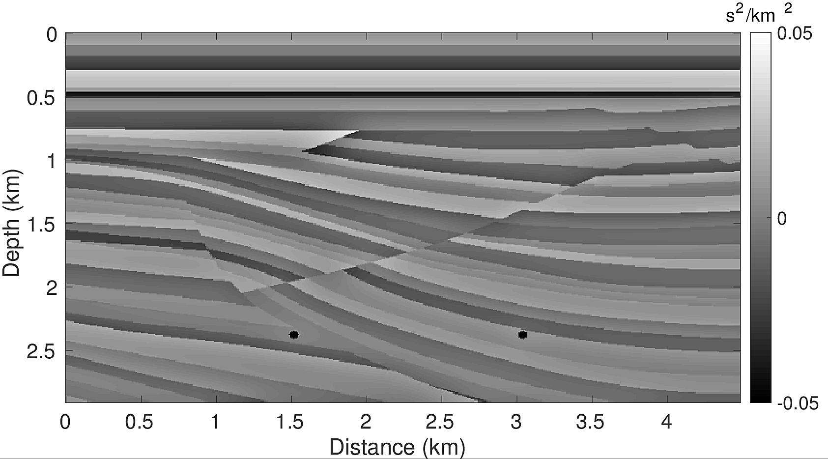
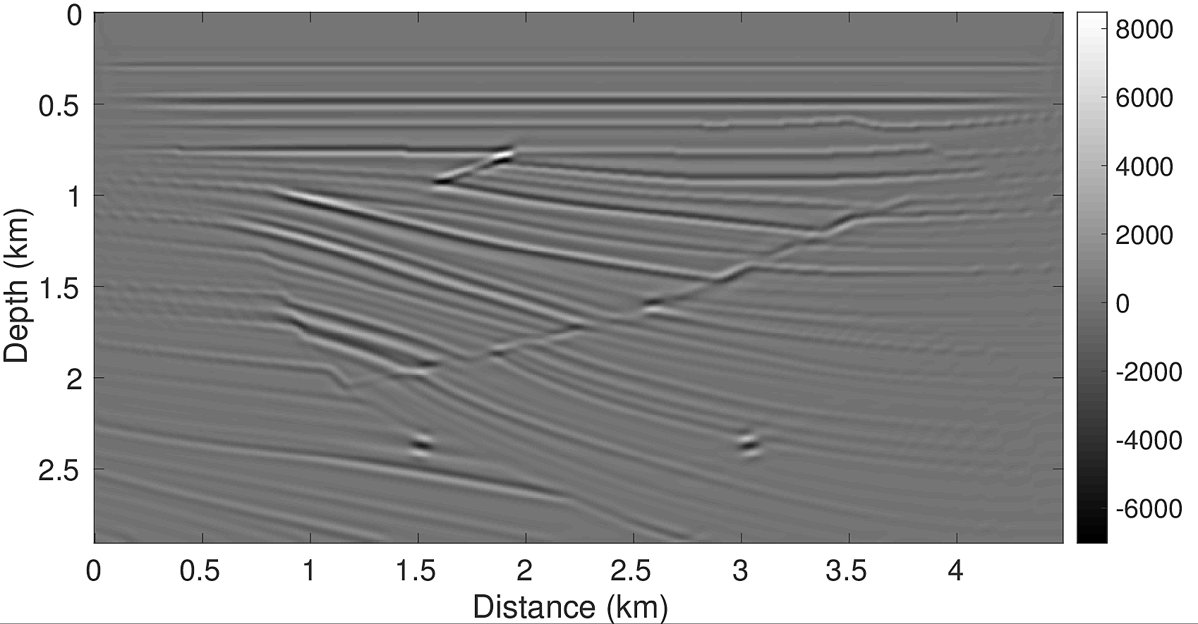
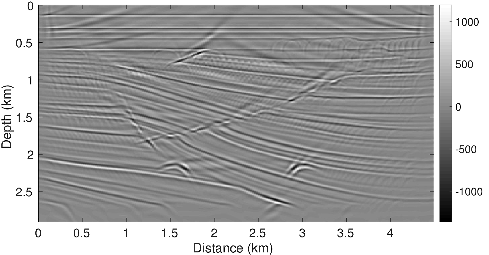
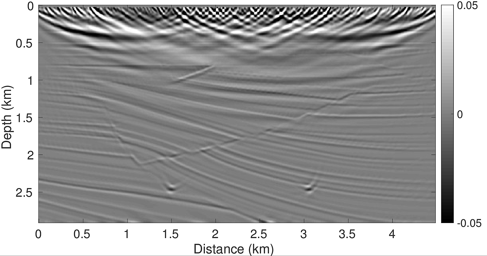
To test our algorithm, we conduct two types of experiments. First, we test the linearized Bregman method for sparsity promoting LS-RTM for the case with a known wavelet \(q\) and a wrong wavelet \(q_0\). We then compare these results with an example in which the source function is unknown and estimated in the described way. For the experiments, we use the top left part of the SIGSBEE2A model, which is 2918m by 4496m and discretized with a grid size of \(7.62\mathrm{m}\) by \(7.62\mathrm{m}\). The model perturbation, which is the difference between the true model and a smoothed background model, is shown in Figure 1a. We generated linearized, single scattered data using the born modelling operator. The experiment consists of \(295\) shot positions with 4 seconds recording time. Each shot is recorded by \(295\) evenly spaced receivers at a depth of \(7.62\mathrm{m}\) and a receiver spacing of \(15.24\mathrm{m}\), yielding a maximum offset of \(4\mathrm{km}\). For later comparisons with the LS-RTM images, we also generate a traditional RTM image (Figure 1b), which illustrates the wrong amplitudes and blurred shapes at interfaces and diffraction points that are typically associated with RTM images. Using a wrong source wavelet in RTM enhances artifacts even more and destroys the energy’s focusing at reflectors and diffractors, as shown in Figure 1c. The wrong wavelet is the initial guess plotted with red line in Figure 3.

In our LS-RTM experiments, we perform 40 iterations and in each iteration draw 8 randomly selected shots. Therefore, after 40 iterations, approximately all shot gathers have been used one time (~one pass through the data). To accelerate the convergence, we apply a depth preconditioner to the model updates, which compensates for the spherical amplitude decay (Herrmann et al., 2008).

LS-RTM with linearized Bregman

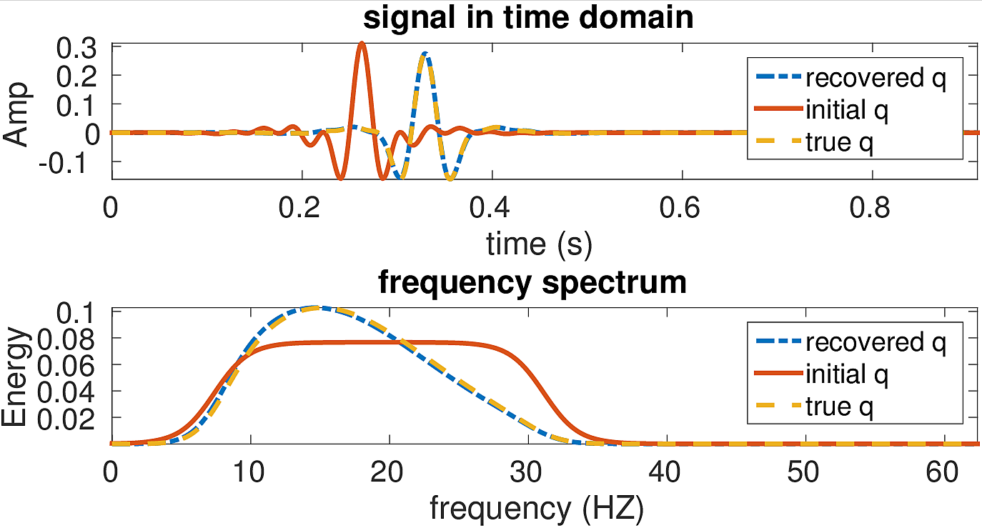
In our first test, we perform LS-RTM via the linearized Bregman method using both a correct source wavelet \(q\) (dashed yellow line, Figure 3) and a wrong wavelet \(q_0\) (solid red line, Figure 3). The true source wavelet \(q\) is formed by convolving a 15 Hz Ricker wavelet with the wavelet \(q_0\), which has a spectrum with a flat shape ranging from 12 to 28 Hz and exponential tapering between 0~12HZ and 28~40HZ (solid red line, Figure 3 bottom).

The only parameter that needs to be provided by the user for the algorithm, is the weighting parameter \(\lambda\). In our experiments, we determine \(\lambda\) in the first iteration, by setting \(\lambda = 0.1\ast\mathsf{max}(\vert \vector{z} \vert)\), which allows roughly 90 percent of the entries in \(\vector{z}\) to pass the soft thresholding in the first iteration. Thresholding too many entries of \(\vector{z}\) leads to slower convergence and more iterations, whereas a value of \(\lambda\) that is too small allows noise and subsampling artifacts to pass the thresholding.

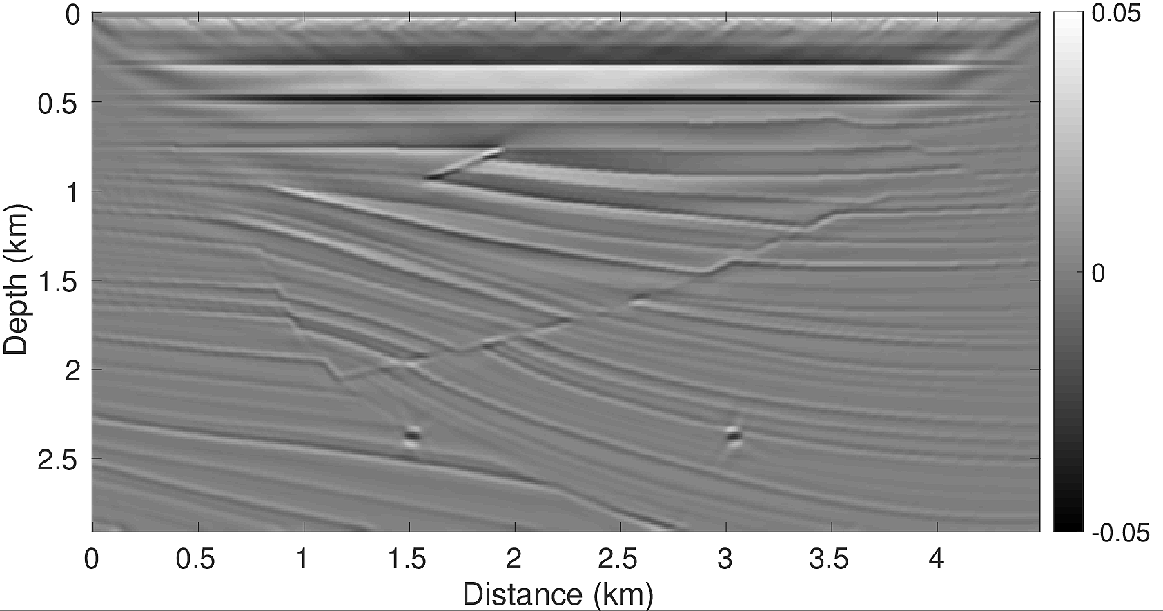
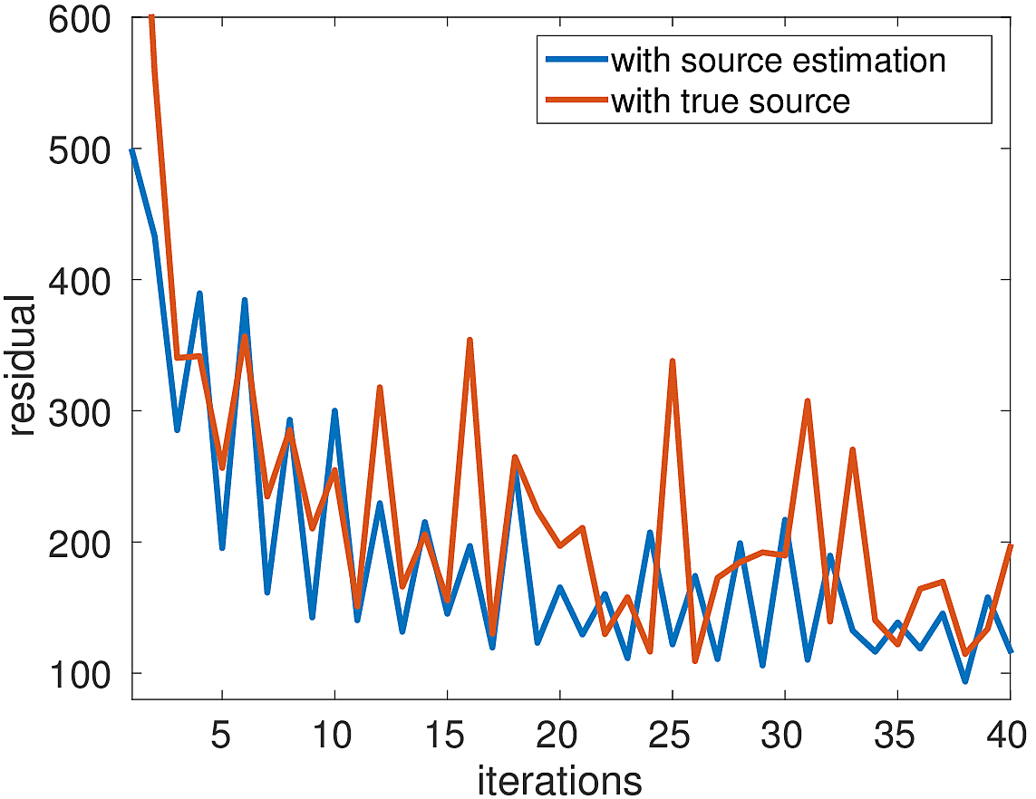
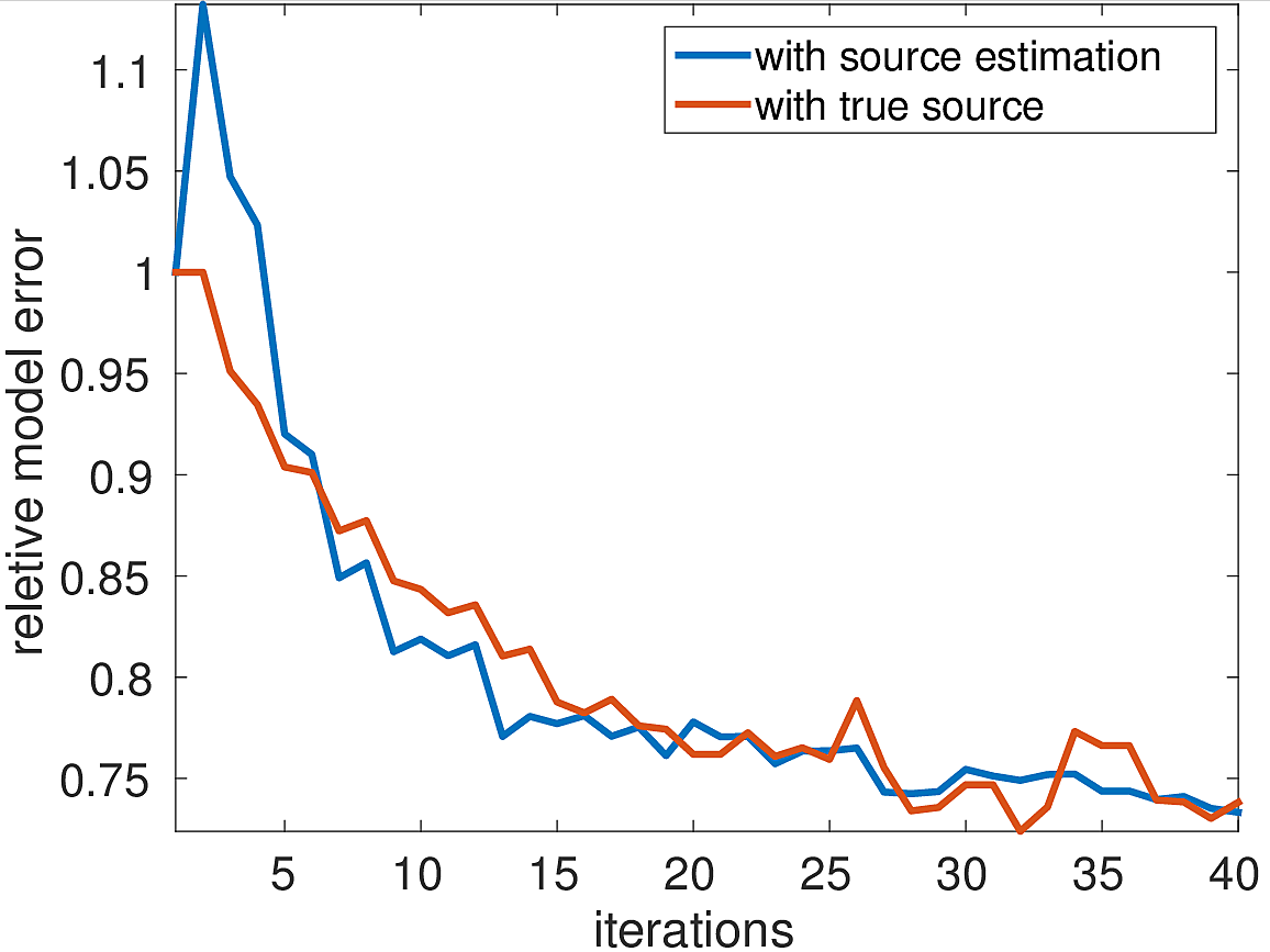
The inversion result of the first experiment with the correct source wavelet is shown in Figure 2a. It clearly shows that the faults and reflectors are all accurately imaged. The interfaces are sharp because the influence of the source wavelet has been removed by the inversion. The data residual decays as a function of the iteration number (Figure 4a), although some jumps occur due to redrawing the shot records in iteration. The model error (Figure 4b) shows the same behaviour. The LS-RTM image with the wrong wavelet on the other hand has strong artifacts, blurred layers and the wrongly located diffractors, as shown in Figure 2c. This test indicates the importance of the correct source in LS-RTM.

Linearized Bregman with source estimation

To solve the problem with the unknown source wavelet, we use the linearized Bregman method with source estimation as described in algorithm 2. The initial guess for the source wavelet \(q_0\) is shown in Figure 3. For the source estimation, the user also needs to supply the parameter \(\alpha\) in the damping function (equation \(\ref{Weight}\)). From our experience, once \(\alpha\) is big enough, the recovered source is not sensitive to the change of \(\alpha\). In our test, we set \(\alpha =8\) and \(\lambda_2=1\). The recovered source (blue dash line) closely matches the correct source time function, but some small differences remain in the frequency spectrums.

With the same strategy for choosing \(\lambda\) as in experiment 1, the inversion result shown in Figure 2c looks as good as the result from the first experiment in which the correct source was used. The residual as a function of the iterations (Figure 4a) is similar to the residual function with the correct source, with the beginning being slightly larger due to the wrong initial guess wavelet. The same is true for the model error in Figure 4b. However, after 40 iterations, both the final data residual and model error are in the range as the residual and error from the experiment with the correct source wavelet.

Conclusions

In this work, we perform sparsity promoting LS-RTM in the time-domain using the linearized Bregman method. This algorithm is easy to implement and allows to work with random subsets of data, which allows to significantly reduce the cost of LS-RTM. We provide an example in which we show that we are able to obtain a sharp image without the imprint of the wavelet and true amplitudes at moderate computational cost, which is in the range of one conventional RTM image. Furthermore, this method allows to incorporate source estimation into the inversion, by solving an small additional least-squares subproblem in each Bregman iteration. We propose a modified version of the LB algorithm including source estimation and show that the image we obtain is as good as the LS-RTM result in which we use the correct source wavelet.

Acknowledgements

We would like to acknowledge Mathias Louboutin for sharing the time stepping finite difference modeling code. This work was financially supported in part by the Natural Sciences and Engineering Research Council of Canada Collaborative Research and Development Grant DNOISE II (CDRP J 375142-08). This research was carried out as part of the SINBAD II project with the support of the member organizations of the SINBAD Consortium.