Phase velocity error minimizing scheme for the anisotropic pure P-wave equation

Philipp A. Witte¹*, Christiaan C. Stolk² and Felix J. Herrmann^1
1Seismic Laboratory for Imaging and Modeling (SLIM), University of British Columbia
²Korteweg-de Vries Institute for Mathematics, University of Amsterdam

Introduction

In the context of migration and full-waveform inversion (FWI), anisotropy is commonly modeled under the acoustic approximation with either pseudo-acoustic wave equations or pure P-wave equations. Most equations are derived from the P-SV dispersion relation by setting the S-wave velocity along the symmetry axis to zero (Alkhalifah, 2000) and by factoring the resulting relation into a system of coupled first- or second-order equations (e.g. Du et al., 2008; Hestholm, 2009; Fowler et al., 2010). Alternatively, some authors have derived pseudo-acoustic wave equations directly from the equation of motion and Hook’s law (Duveneck and Bakker, 2011; Y. Zhang et al., 2011).

Pure P-wave equations have been developed as an elegant approach to deal with S-wave artifacts that appear in all of these pseudo-acoustic wave equations. The artifacts not only affect migrated images optically, but can also lead to stability issues of the modeling schemes. Pure P-wave equations are obtained by factoring the pseudo-acoustic dispersion relation into separate P- and S-wave terms, which leads to an equation that contains the square root of a differential operator (Liu et al., 2009). Due to this operator, the pure P-wave equation cannot be turned directly into a modeling scheme and is most easily approximated by expanding the square-root into a first-order Taylor series and by further simplification of the anellitpic term. The resulting equation is completely free of S-wave artifacts and has no stability restrictions on the Thomsen parameters and has therefore gained a large popularity in context of anisotropic RTM (Etgen and Brandsberg-Dahl, 2009; Crawley et al., 2010a, 2010b; Chu et al., 2011; Zhan et al., 2013). The main drawbacks of this “standard” pure P-wave equation are a more difficult discretization and kinematic errors introduced by the approximations. To lower these errors, several authors have proposed equations with higher order series expansions of the square root operator and/or the anelliptic term (R. Pestana et al., 2012; Chu et al., 2013; Du et al., 2014). All these approaches lower the phase velocity error, but come at increasing computational cost. Further notable alternatives include Padé approximations of the square root operator (Schleicher and Costa, 2015), low-rank approximations (Song et al., 2013; Fomel et al., 2013) and optimized low-rank approximations (Wu and Alkhalifah, 2014).

In this paper, we obtain a pure P-wave equation by a different approach, namely by approximating the exact pure P-wave equation through a polynomial expansion. The coefficients of the expansion are obtained by solving an optimization problem that minimizes the phase velocity errors for a given range of Thomsen parameters and phase angles. We show that the phase velocity errors of this scheme are not only significantly smaller than the errors of the “standard” pure P-wave equation, but are in fact in the range of second-order Taylor approximations of exact pure P-wave equation. Furthermore, the computational cost (in terms of FFTs per time step) is the same as the “standard” pure P-wave equation scheme by Chu et al. (2011), which makes this approach feasible for large scale applications.

Pure P-wave equations in TI media

The derivations for any of the pure P-wave equations start from the pseudo-acoustic dispersion relation, which is obtained by setting the S-wave velocity in the coupled P-SV dispersion relation to zero (Alkhalifah, 2000) and by factoring the result into two separate equations for P-waves and SV-waves (Liu et al., 2009). The exact pure P-wave relation is: \[ \begin{equation} \begin{aligned} &-\frac{\omega^2}{v_{pz}^2} = -\frac{1}{2} \Big[(1+2\epsilon)(k_x^2+k_y^2) + k^2_z \Big] \\ &- \frac{1}{2}\sqrt{\Big[ (1+2\epsilon)(k_x^2+k_y^2) + k^2_z\Big]^2 + 8(\delta-\epsilon)(k_x^2+k_y^2)k_z^2}, \end{aligned} \label{pureP2} \end{equation} \] where \(\omega\) is the angular frequency, \(k_{x,y,z}\) are the spatial wave numbers in the \(x,y,z\) direction and \(v_{pz}\) is the vertical P-wave velocity. Since this equation contains the square root of a differential operator, a time-domain scheme cannot be derived from this formulation directly. Liu et al. (2009) use an optimized separable approximation to solve Equation \(\ref{pureP2}\). A more convenient approach was proposed by Chu et al. (2011), in which the authors approximate the square root into a first-order Taylor series and simplify the anellipticity term, which yields the standard pure P-wave equation: \[ \begin{equation} -\frac{\omega^2}{v_{pz}^2} \approx - \Big[ (1+2\epsilon)(k_x^2+k_y^2)+k^2_z \Big] - \frac{2(\delta-\epsilon)(k_x^2+k_y^2)k_z^2}{k^2} \label{purePexpand3} \end{equation} \] with \(k^2=k_x^2+k_y^2+k^2_z\) . The equation can be easily solved with the pseudo-spectral method, but comes at the cost of kinematic inaccuracies for strong non-ellipticity. In a follow-up paper, Chu et al. (2013) investigate this further and suggest an alternative formulation in which the anelliptic term is represented through a geometric series: \[ \begin{equation} \begin{aligned} -\frac{\omega^2}{v_{pz}^2} \approx &- \Big[ (1+2\epsilon)(k_x^2+k_y^2)+k^2_z \Big] \\ &-\frac{2(\delta-\epsilon)(k_x^2+k_y^2)k_z^2}{k^2} \sum^{M}_{m=0} \Bigg( -2\epsilon\frac{k_x^2+k_y^2}{k^2} \Bigg)^m \end{aligned} \label{purePseries} \end{equation} \] For \(M=0\), Equation \(\ref{purePseries}\) reduces to Equation \(\ref{purePexpand3}\), whereas more expansion terms lead to a smaller error at a larger computational cost.

Phase velocity error minimizing pure P-wave equation

Instead of a Taylor expansion of the square root, we approximate Equation \(\ref{pureP2}\) using a polynomial expansion with coefficients \(a_j \in \mathbb{R}~\): \[ \begin{equation} \begin{aligned} -\frac{\omega^2}{v_{pz}^2} \approx & a_1 k^2 + a_2 \Big( (k_x^2+k_y^2)-k^2_z \Big) + a_3 \frac{\Big( (k_x^2+k_y^2)-k^2_z \Big)^2}{k^2} \\ + & a_4 \frac{\Big( (k_x^2+k_y^2)-k^2_z \Big)^3}{(k^2)^2} \end{aligned} \label{expansion} \end{equation} \] The coefficients \(a_j\) are determined such that they minimize the phase velocity error of this scheme. These coefficients are a function of the Thomsen parameters and for now we set \(\epsilon,\delta=const\) and \(v_{pz}=1\). The scalar phase velocity is given by \(v_{ph} = \frac{\omega}{||k||}\) and we define \(k=1\) and \[ \begin{equation} k_z^2(\alpha) = \cos^2 \alpha \label{kz} \end{equation} \] \[ \begin{equation} k_x^2(\alpha) + k_y^2(\alpha) = k_r^2(\alpha) = \sin^2 \alpha, \label{kr} \end{equation} \] where \(\alpha \in [0,\frac{\pi}{2}]\)is the phase angle. With these definitions, the (squared) phase velocity of our approximated P-wave equation is given by: \[ \begin{equation} \begin{split} v_{approx}^2(\alpha, a_1, a_2, a_3, a_4) = \Bigg( a_1 + a_2\Big[ k_r^2(\alpha) - k^2_z(\alpha) \Big] \\ + a_3\Big[ k_r^2(\alpha) - k^2_z(\alpha) \Big]^2 + a_4\Big[ k_r^2(\alpha) - k^2_z(\alpha) \Big]^3 \Bigg) \end{split} \label{newPhase} \end{equation} \] The phase velocity of the exact pure P-wave equation is given accordingly to Equation \(\ref{pureP2}\) . The objective function to be minimized in order to calculate the coefficients \(a_j\) is the relative phase velocity error \[ \begin{equation} E(a_1,a_2,a_3,a_4) =\sqrt{ \frac{v_{approx}^2(\alpha, a_1, a_2, a_3, a_4)}{v_{true}^2(\alpha)}} - 1 \label{phaseError} \end{equation} \] The ratio of the squared velocities is going to be very close to \(1\), so we do a first-order Taylor approximation of \(\sqrt{x}\) at \(x=1\), which leads to:\(\sqrt{x}-1 \approx \frac{1}{2}(x-1)\). By doing so, the error depends linearly on the coefficients \(a_j\) and the optimal coefficients that minimize the error are given as the solution of a linear least squares problem: \[ \begin{equation} a_j = \underset{a_j}{\operatorname{argmin}} \hspace{0.2cm} \int\limits_{0}^{\frac{\pi}{2}} \left|\left| \frac{1}{2} \Big( \frac{v_{approx}^2(\alpha, a_1, a_2, a_3, a_4)}{v_{true}^2(\alpha)} - 1 \Big)\right|\right|^2 d\alpha \label{leastSquares} \end{equation} \]

Extension to varying anisotropy parameters

Solving the least squares problem in Equation \(\ref{leastSquares}\) gives coefficients that are optimized for a particular value of \(\epsilon\) and \(\delta\). In general, we are interested in modeling wave propagation in media with spatially varying \(\epsilon\) and \(\delta\), where \(\epsilon,\delta \in \mathbb{R}\) and the parameters lie in some (physically constrained) range \([\epsilon_{min},\epsilon_{max}]\) and \([\delta_{min},\delta_{max}]\). Rather than calculating (and storing) all \(a_j(\epsilon,\delta)\) for every combination of \(\epsilon\) and \(\delta\) in the model, we approximate the functions \(a_j(\epsilon,\delta)\) by interpolation with Legendre polynomials: \[ \begin{equation} a_j = p_{jkl} L_k(\epsilon)L_l(\delta), \label{interpol} \end{equation} \] where \(j=1,...,4\) is the coefficient number and \(L_k\) are the Legendre polynomials of order \(k\) and we use polynomials up to 3rd order \((k,l=0,...,3)\).

Instead of solving for the four coefficients \(a_j\) that minimize the phase velocity error for a given set of phase angles and \(\epsilon,\delta=const.\), we now solve for \(4^3=64\) coefficients \(p_{jkl}\) that minimize the phase velocity error for a given set of \(\epsilon,\delta\) values and a set of phase angles \(\alpha\). Optimizing for the values \(p_{jkl}\) is still a linear least squares problem. We simply replace the coefficients \(a_j\) in Equation \(\ref{newPhase}\) and solve the following least squares problem, in which the approximated phase velocity is now a function of the phase angle, Thomsen parameters and coefficients \(p_{jkl}\): \[ \begin{equation} \small p_{jkl} = \small \underset{p_{jkl}}{\operatorname{argmin}} \hspace{0.2cm} \int\limits_{\epsilon_{min}}^{\epsilon_{max}} \int\limits_{\delta_{min}}^{\delta_{max}} \int\limits_{0}^{\frac{\pi}{2}} \left|\left| \frac{1}{2} \Big( \frac{ v_{approx}^2(\alpha, \epsilon, \delta, p_{jkl}) }{v_{true}^2(\alpha,\epsilon,\delta)} - 1 \Big)\right|\right|^2 d\alpha \hspace{0.1cm} d\delta \hspace{0.1cm} d\epsilon \label{leastSquares2} \end{equation} \] The size of this linear system is fairly small (\(64\) unknowns and \(20^3\) observations if we use \(20\) angles and Thomsen parameters each) and can be solved using QR decomposition or other fast direct methods.

Phase velocity error analysis

To evaluate the accuracy of the optimized pure P-wave relation, we plot the relative phase error (Equation \(\ref{phaseError}\)) and compare it to the errors from the pure P-wave equation from Chu et al. (2013) (Equation \(\ref{purePseries}\)) for a different number of expansion terms \(M=0,1,2\). For further comparison, we also plot the error of the second order Taylor expansion of Equation \(\ref{pureP2}\) (Chu et al., 2011): \[ \begin{equation} \begin{aligned} -\frac{\omega^2}{v_{pz}^2} \approx - & \Big[ (1+2\epsilon)(k_x^2+k_y^2)+k^2_z \Big] - \frac{2(\delta-\epsilon)(k_x^2+k_y^2)k_z^2}{(1+2\epsilon)(k_x^2+k_y^2)+k^2_z} \\ + & \frac{\Big[2(\delta-\epsilon)(k_x^2+k_y^2)k_z^2\Big]^2}{\Big[(1+2\epsilon)(k_x^2+k_y^2)+k^2_z\Big]^3} \end{aligned} \label{pureP2ndorder} \end{equation} \] For our optimized scheme, we first define a range for the Thomsen parameters and we calculate the optimized coefficients \(p_{jkl}\) using \(20\) evenly spaced values of \(\epsilon\) and \(\delta\) within that range. We choose \(\epsilon \in [0,0.5]\) and \(\delta \in [-0.1,0.4]\), which are typical ranges for the Thomsen parameters (Thomsen, 1986). Furthermore, we use \(20\) phase angles within the range from \(0\) to \(\frac{\pi}{2}\). With the optimized coefficients, the phase velocity for any combination of \(\epsilon\) and \(\delta\) can be calculated as a function of the phase angle. Figures 1 and 2 show the phase velocity errors for two different combinations of Thomsen parameters.

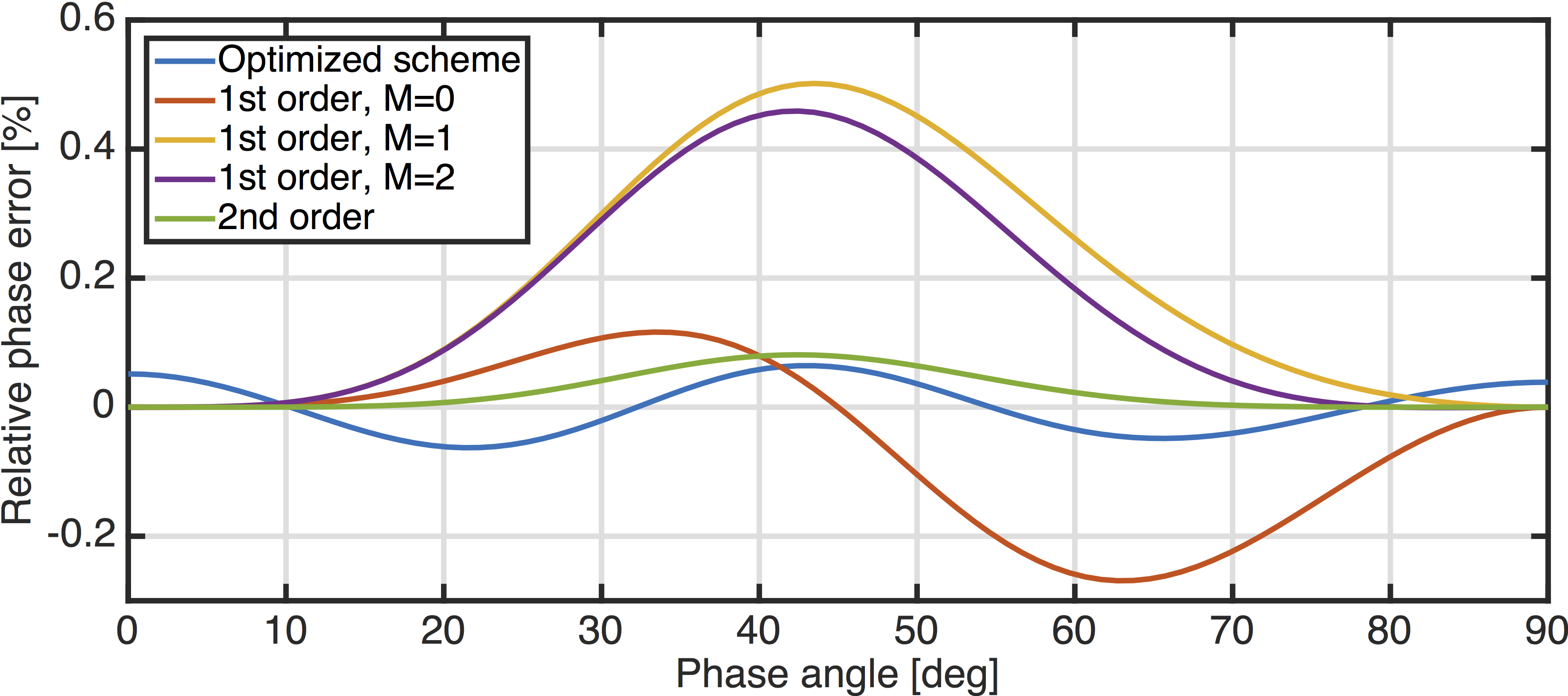
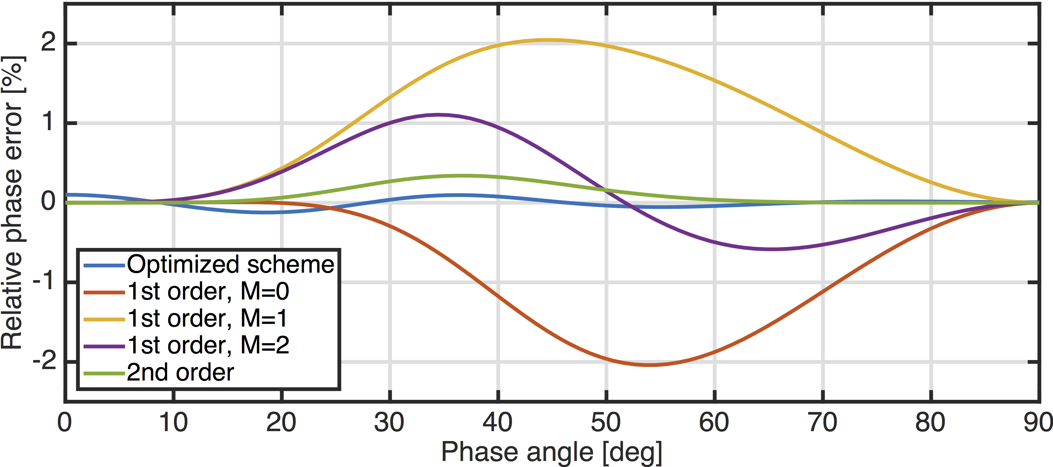
In both examples, the phase error from the optimized scheme is smaller than any of the other errors, in particular, the optimized scheme is even more accurate than the second order expansion from Equation \(\ref{pureP2ndorder}\). Because the coefficients of the expansion terms are calculated such that they minimize the phase error in a least squares sense, the error is distributed along all phase angles, whereas the other schemes based on Taylor expansions are exact at \(\alpha=0\) and \(90\) degree, but inaccurate at intermediate angles.

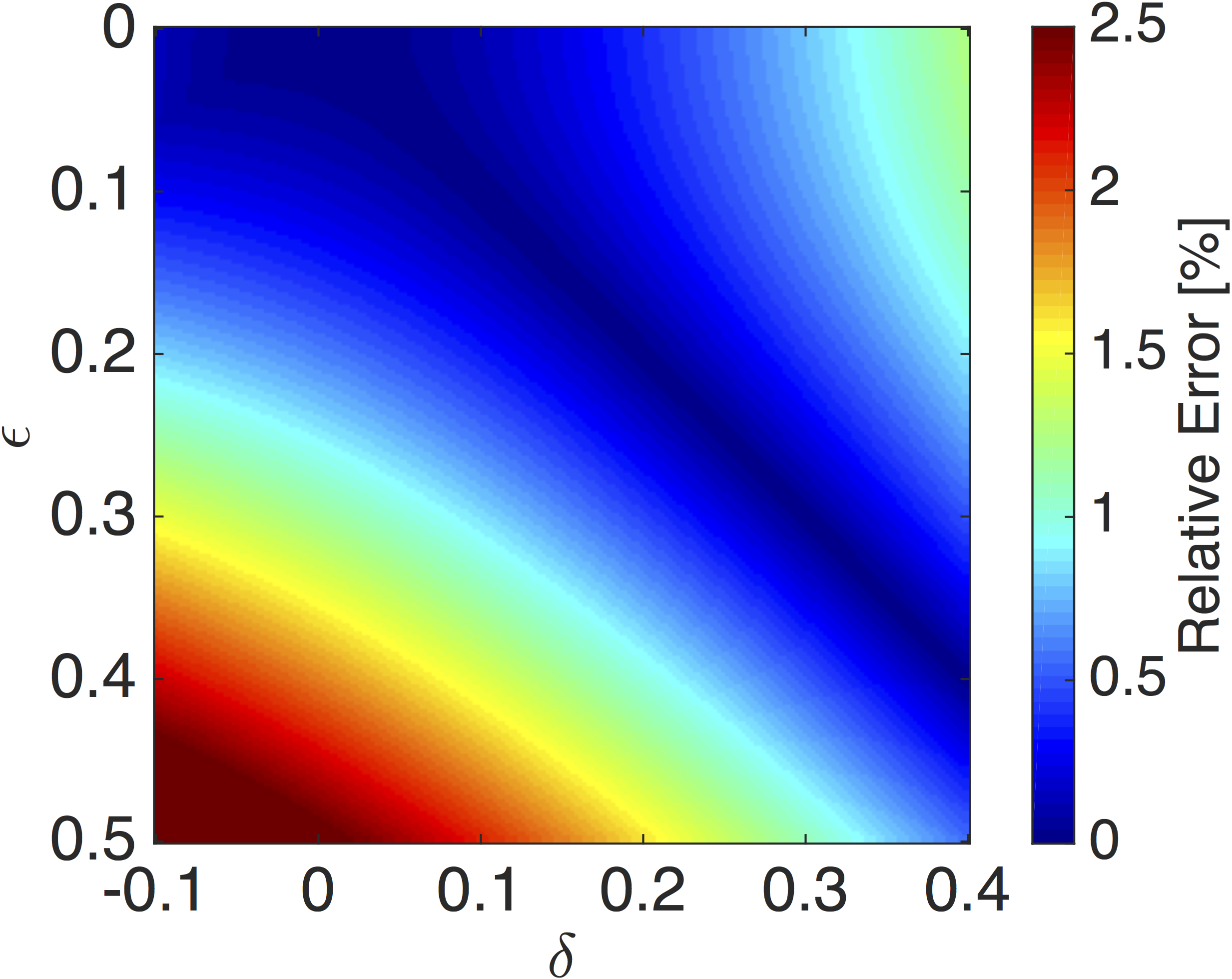
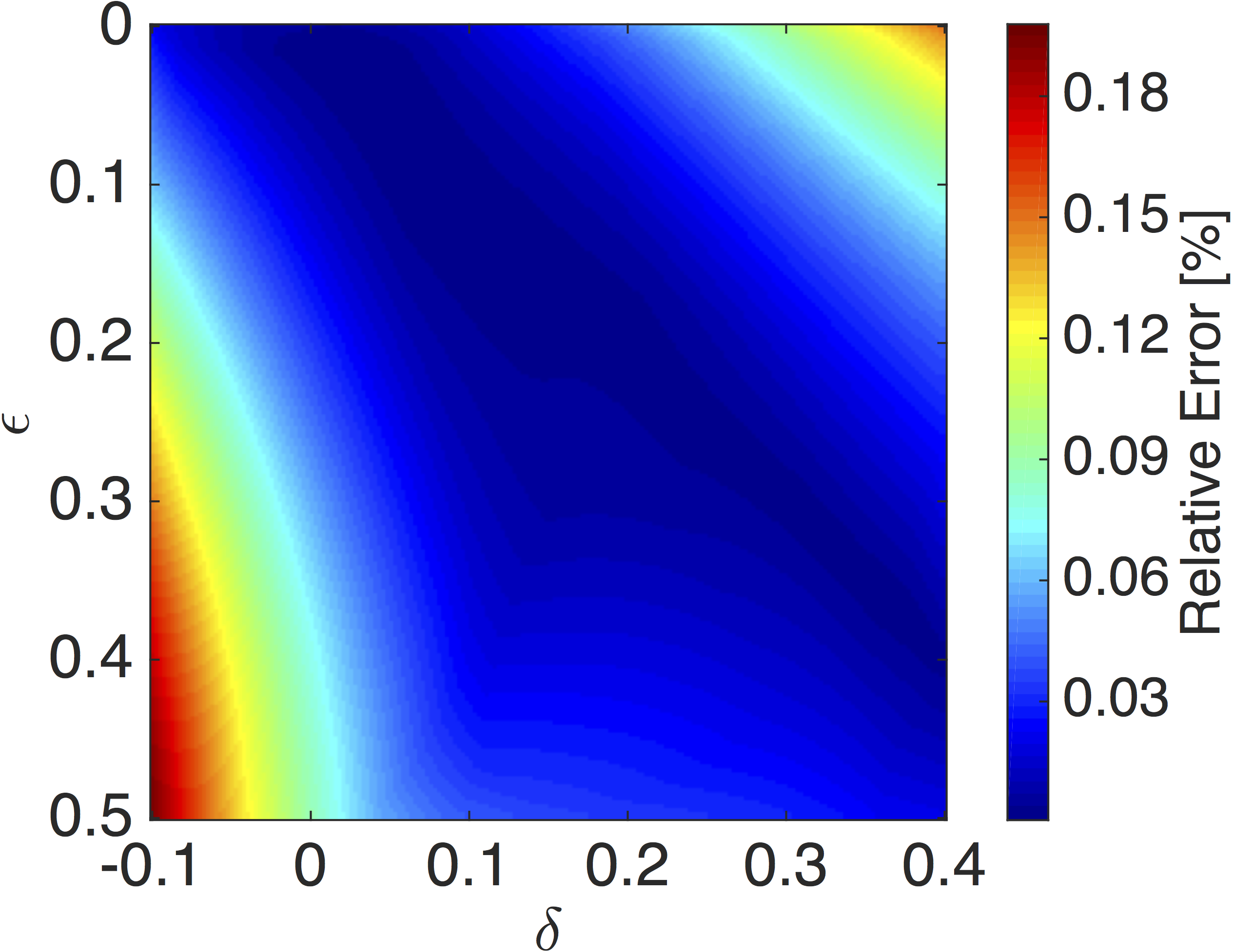
Furthermore, the error is calculated as a function of \(\epsilon\) and \(\delta\): \[ \begin{equation} E(\epsilon,\delta) = \max{\Big(|E(\epsilon,\delta,\alpha)|\Big)} \label{epsErr} \end{equation} \] As expected, the error for both approximations is small for \(\epsilon\approx\delta\) and becomes larger as the difference between the parameters increases (Figure 3). The phase error of our optimized scheme is less than \(0.2\) percent within the entire \(\epsilon,\delta\) range, whereas the phase velocity error of the standard pure P-wave equation is already larger than \(1\) percent for a large part of the \(\epsilon, \delta\) range and larger than 2 percent for highly non-elliptic media. For large velocity models, where waves are often propagated for more than a hundred wavelengths, seismic data modeled with the standard pure P-wave equation is potentially cycle skipped in certain directions, which then results in misplaced reflectors in migrated images or wrong gradient updates for FWI.

Forward Modeling scheme

For a VTI medium, the optimized dispersion relation can be directly turned into a time-wavenumber equation: \[ \begin{equation} \begin{aligned} \frac{1}{v_{pz}^2}\frac{\partial^2 P}{\partial t^2} = & p_{1kl}L_k(\epsilon)L_l(\delta) \mathcal{F}^{-1} \Big\{ k^2\bar{P} \Big\} \\ + & p_{2kl}L_k(\epsilon)L_l(\delta) \mathcal{F}^{-1}\Big\{ (k_x^2 + k_y^2 - k_z^2)\bar{P} \Big\} \\ + & p_{3kl}L_k(\epsilon)L_l(\delta) \mathcal{F}^{-1} \Bigg\{ \frac{(k_x^2 + k_y^2 - k_z^2)^2}{k^2}\bar{P} \Bigg\} \\ + & p_{4kl}L_k(\epsilon)L_l(\delta) \mathcal{F}^{-1} \Bigg\{ \frac{(k_x^2 + k_y^2 - k_z^2)^3}{k^4}\bar{P} \Bigg\} + S(t), \end{aligned} \label{PSscheme} \end{equation} \] where \(P\) is the wavefield in the physical domain, \(\bar{P}\) is the wavefield in the wavenumber domain, \(\mathcal{F}^{-1}\) is the three-dimensional inverse Fourier transform and \(S(t)\) is the source function.

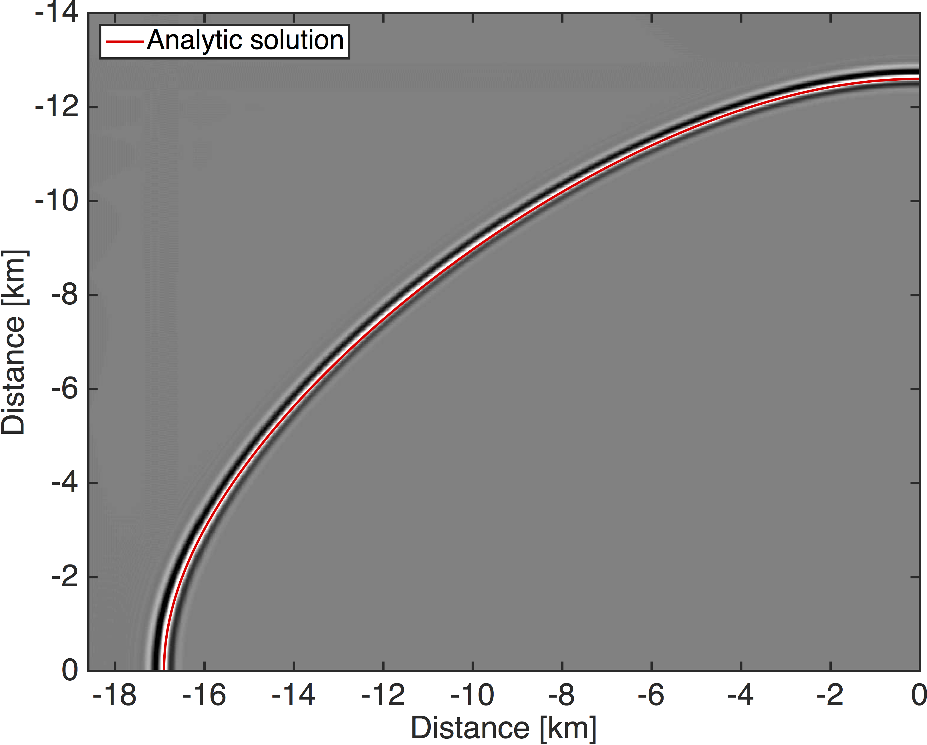
Figure 4 show the wavefronts after propagating a \(15\,\mathrm{Hz}\) Ricker wavelet in a homogeneous 2D medium with \(v_{pz}=2 \mathrm{kms^{-1}}\), \(\epsilon=0.4\) and \(\delta=-0.05\) for \(6.5\) seconds. This corresponds to propagating the source wavelet for approximately \(100\) wavelengths and the wavefront of the analytical solution is overlaid onto the wavefield snapshots. The wavefront of the standard pure P-wave equation is correct at \(0\) and \(90\) degrees, but differs for more than a wavelength from the analytical solution at intermediate phase angles. In the context of FWI, this means that the modeled data is possibly cycle skipped, even if the correct velocity model was used. The wavefront that is modeled with the optimized equation on the other hand, closely matches the analytical solution for all phase angles.

The optimized pure P-wave equation can be extended to TTI media as well by replacing the wavenumber vectors with locally rotated vectors \(\hat{k}_{x,y,z}\) that are tilted at an angle \(\theta\) against the vertical axis and horizontally rotated with the azimuth \(\phi\). In the time-domain scheme, these spatially varying angles need to be separated from the wavenumber terms, which potentially increases the number of terms in Equation \(\ref{PSscheme}\) enormously. However, due to the special structure of the optimized equation, the right-hand side of Equation \(\ref{PSscheme}\) can be calculated recursively: \[ \begin{equation} u_1 = \Big\{ \mathcal{F}^{-1} k^2 \Big\} \bar{P} \label{PSscheme1} \end{equation} \] \[ \begin{equation} \begin{aligned} u_2 = \Big\{ &c_1 \mathcal{F}^{-1} k_x^2 + c_2 \mathcal{F}^{-1} k_y^2 + c_3 \mathcal{F}^{-1} k_z^2 \\ + &c_4 \mathcal{F}^{-1} k_x k_y + c_5 \mathcal{F}^{-1} k_x k_z +c_6 \mathcal{F}^{-1} k_y k_z \Big\} \bar{P} \end{aligned} \label{PSscheme2} \end{equation} \] \[ \begin{equation} \begin{aligned} u_3 = \Big\{ &c_1 \mathcal{F}^{-1} \frac{k_x^2}{k^2} + c_2 \mathcal{F}^{-1} \frac{k_y^2}{k^2} + c_3 \mathcal{F}^{-1} \frac{k_z^2}{k^2} \\ + &c_4 \mathcal{F}^{-1} \frac{k_x k_y}{k^2} + c_5 \mathcal{F}^{-1} \frac{k_x k_z}{k^2} + c_6 \mathcal{F}^{-1} \frac{k_y k_z}{k^2} \Big\} \mathcal{F} u_2 \end{aligned} \label{PSscheme3} \end{equation} \] The last term \(u_4\) is calculated from \(u_3\) in the same way as \(u_3\) from \(u_2\). The \(c_i\) terms contain the spatial tilt and rotation of the symmetry axis: \[ \begin{equation} \begin{aligned} &c_1 = 1-2\sin^2{\theta}\cos^2{\phi};\hspace{0.2cm} c_2 = 1-2\sin^2{\theta}\sin^2{\phi} \\ \\ &c_3 = - \cos{2\theta}; \hspace{0.2cm} c_4 = - 2 \sin^2{\theta} \sin{2\phi} \\ \\ &c_5 = - \sin{2\theta} \cos{\phi}; \hspace{0.2cm} c_6 = - \sin{2\theta} \sin{\phi} \end{aligned} \label{c1} \end{equation} \] The last step is to sum and multiply these terms with the optimized coefficients \(p_{jkl}\): \[ \begin{equation} \begin{aligned} \frac{1}{v_{pz}^2}\frac{\partial^2 P}{\partial t^2} = &p_{1kl}L_k(\epsilon)L_l(\delta) u_1 + p_{2kl}L_k(\epsilon)L_l(\delta) u_2 \\ + &p_{3kl}L_k(\epsilon)L_l(\delta) u_3 + p_{4kl}L_k(\epsilon)L_l(\delta) u_4 + S(t), \end{aligned} \label{PSscheme5} \end{equation} \] Overall, the right-hand side of Equation \(\ref{PSscheme5}\) can be calculated at the cost of 3 FFTs and 19 inverse FFTs in a 3D TTI medium, which is the same number of FFTs as in the standard pure P-wave equation (Chu et al., 2011).

Conclusions

In this work, we introduce a novel approach to approximate the pure P-wave dispersion relation and derive a time-stepping scheme for acoustic-anisotropic modeling. Rather than using Taylor expansions, we approximate the exact P-wave relation with a scheme that minimizes the relative phase velocity error in a least squares sense. This approach yields a highly accurate modeling scheme with relative phase velocity errors in the range of a fraction of one percent, making this method an order of magnitude more accurate than other pure P-wave equations. In the context of FWI and migration this ensures that for a correct velocity model, modeled waveforms are not cycle skipped or reflectors are not mispositioned. Furthermore, we provide an efficient implementation of the optimized dispersion relation for TTI media that has similar computational cost as the standard pure P-wave equation and makes this method feasible for 3D computations.

Acknowledgements

This work was financially supported in part by the Natural Sciences and Engineering Research Council of Canada Collaborative Research and Development Grant DNOISE II (CDRP J 375142-08). This research was carried out as part of the SINBAD II project with the support of the member organizations of the SINBAD Consortium.

References

Alkhalifah, T., 2000, An acoustic wave equation for anisotropic media: Geophysics, 65, 1239–1250. doi:10.1190/1.1444815
Chu, C., Macy, B. K., and Anno, P. D., 2011, Approximation of pure acoustic seismic wave propagation in TTI media: Geophysics, 76, WB97–WB107. doi:10.1190/geo2011-0092.1
Chu, C., Macy, B. K., and Anno, P. D., 2013, Pure acoustic wave propagation in transversely isotropic media by the pseudospectral method: Geophysical Prospection, 556–567. doi:10.1111/j.1365-2478.2012.01077.x
Crawley, S., Brandsberg-Dahl, S., and McClean, J., 2010a, 3D TTI RTM using the pseudo-analytic method: 80th Annual International Meeting, SEG, Expanded Abstracts, 3216–3220. doi:10.1190/1.3513515
Crawley, S., Brandsberg-Dahl, S., McClean, J., and Chemingui, N., 2010b, TTI reverse time migration using the pseudo-analytic method: The Leading Edge, 29, 1278–1284. doi:10.1190/1.3517310
Du, X., Fletcher, R. P., and Fowler, P. J., 2008, A new pseudo-acoustic wave equation for VTI media:. EAGE. doi:10.3997/2214-4609.20147774
Du, X., Fowler, P. J., and Fletcher, R. P., 2014, Recursive integral time-extrapolation methods for waves: A comparative review: Geophysics, 79, T9–T26. doi:10.1190/geo2013-0115.1
Duveneck, E., and Bakker, P. M., 2011, Stable P-wave modeling for reverse-time migration in tilted TI media: Geophysics, 76, 65–75. doi:10.1190/1.3533964
Etgen, J. T., and Brandsberg-Dahl, S., 2009, The pseudo-analytical method: Application of pseudo-Laplacians to acoustic and acoustic anisotropic wave propagation: 79th Annual International Meeting, SEG, Expanded Abstracts, 2552–2555. doi:10.1190/1.3255375
Fomel, S., Ying, L., and Song, X., 2013, Seismic wave extrapolation using lowrank symbol approximation: Geophysical Prospecting, 61, 526–536. doi:10.1111/j.1365-2478.2012.01064.x
Fowler, P. J., Du, X., and Fletcher, R. P., 2010, Coupled equations for reverse time migration in transversely isotropic media: Geophysics, 75, S11–S22. doi:10.1190/1.3294572
Hestholm, S., 2009, Acoustic VTI modeling using high-order finite differences: Geophysics, 74, T67–T73. doi:10.1190/1.3157242
Liu, F., Morton, S. A., Jiang, S., Ni, L., and Leveille, J. P., 2009, Decoupled wave equations for P and SV waves in an acoustic VTI media: 79th Annual International Meeting, SEG, Expanded Abstracts, 2844–2848. doi:10.1190/1.3255440
Pestana, R., Ursin, B., and Stoffa, P. L., 2012, Rapid expansion and pseudo spectral implementation for reverse time migration in VTI media: Journal of Geophysics and Engineering, 9. doi:10.1088/1742-2132/9/3/291
Schleicher, J., and Costa, J., 2015, A separable strong-anisotropy approximation for pure qP wave propagation in TI media: 85th Annual International Meeting, SEG, Expanded Abstracts, 3565–3570. doi:10.1190/segam2015-5934948.1
Song, X., Fomel, S., and Ying, L., 2013, Lowrank finite-differences and lowrank Fourier finite-differences for seimsic wave extrapolation in the acoustic approximation: Geophysical Journal International, 193, 960–969. doi:10.1093/gji/ggt017
Thomsen, L., 1986, Weak elastic anisotropy: Geophysics, 51, 1964–1966. doi:10.1190/1.1442051
Wu, Z., and Alkhalifah, T., 2014, The optimized expansion based low-rank method for wavefield extrapolation: Geophysics, 79, T51–T60. doi:10.1190/geo2013-0174.1
Zhan, G., Pestana, R. C., and Stoffa, P. L., 2013, An efficient hybrid pseudospectral/finite-difference scheme for solving the TTI pure P-wave equation: Journal of Geophysics and Engineering, 10. doi:10.1088/1742-2132/10/2/025004
Zhang, Y., Zhang, H., and Zhang, G., 2011, A stable TTI reverse time migration and its implementation: Geophysics, 76, WA3–WA11. doi:10.1190/1.3554411