Frequency down-extrapolation with TV norm minimization

Introduction

We consider acoustic full-waveform inversion (FWI) for a typical situation where low-frequency information is missing. It is well known that the low wavenumber data can effectively reduce the number of local minima of FWI and therefore can be expected to improve the inversion when a bad initial guess of the model is provided. However, missing low-frequency situations are commonly observed in both marine and land acquisitions where data below \(5\,\mathrm{Hz}\) is often too noisy to be useful.

Approaches tackling this problem consists of both data processing techniques and wave-equation based techniques. The former follows the general belief that the raw data has some special structure that can be exploited to extract missing low-frequency information from high frequencies. One common assumption is sparse reflectivity, i.e., the reflectivity series corresponding to a single trace is a sparse spike train. We comment that this is an idealized assumption that does not strictly hold even in a 2D constant medium, let alone when we consider possible frequency dependent dispersion and attenuation effects present in real dataset. As a result, it is important to design a robust extrapolation method, which produces acceptable results when the underlying assumptions are slightly violated and noise is added. Our point here is that we prefer a method that is arguably robust rather than relying on unrealistic assumptions to create what seems like superior but in practice infeasible results.

Many methods have been proposed for broadening the spectrum. In the work by Xie (2013), the author proposed to isolate single events by windowing in combination with making a linear phase assumption to extend the spectrum. Unfortunately, the requirement of manually selecting windows prevents this approach from effectively handling complex models where two overlapping event cannot visually separated. (Taylor and McCoy, 1979), on the other hand, uses a convex optimization approach that minimizes the data misfit plus the \(\ell_1\)-norm of the Green’s function. In the light of recent results in super-resolution in the field of Compressed Sensing (Candes and Fernandez-Granda, 2014; Demanet and Nguyen, 2015), this approach is better understood. In particular, it is now known that this approach is sensitive to discretization errors and is also known to give erroneous results when impulsive arrivals (spikes) of opposite signs are too closely (closer than twice the shortest wavelength) located.

More recently, Li and Demanet (2016) proposed a new method, which for the first time explores the inter-trace relationships. To arrive at their results, the authors use the Multiple Signal Classification (MUSIC) algorithm (Schmidt, 1986) to deconvolve traces with only a few events, followed by a lateral continuous extension of these events to the nearby traces while keeping feasibility of the data. Due to the use of the MUSIC algorithm, this method is immune to discretization errors and the benefits of continuation amongst traces in the lateral direction has been clearly demonstrated by their stylized examples.

The missing low-frequency treatment in the wave-equation based approaches, on the other hand, seek to modify the inversion procedure itself with the hope of increasing the convexity of the optimization problem, leading to variants of FWI (Wu Ru-Shan et al., 2013; Hu, 2014; Sun and Symes, 2012; Van Leeuwen and Herrmman, 2013; Warner and Guasch, 2013; Biondi and Almomin, 2014). These methods still have the true model as the global minimum, hence more stable than the extrapolation based techniques. However, they are perhaps less intuitive and the performance may sometimes be hard to predict.

In this abstract, we revisit the convex optimization approach as a frequency extrapolation method in the data processing regime. We propose to use a TV norm regularizer that takes into account the spatial correlation among traces. Comparing to the original \(\ell_1\) regularizer (Taylor and McCoy, 1979), our method has the added benefit of increased stability and speed as well as robustness to the discretization. It should be noted that this method is only intended for extrapolating towards the lower end of the spectrum, not to the higher end nor intended to recovering the complete Green’s function.

Methodology

Under the no dispersion and no attenuation assumption, a single seismic trace \(d_j\) with \(m\) events can be written as \[ \begin{equation} \begin{aligned} & d_j(t)= q(t)*G_j(t), \quad \quad \ \ j=1,...,nr, \\ & G_j(t)=\sum\limits_{i=1}^m a_{i}^j \chi (t-t_i^j), \quad i=1,...,m, \end{aligned} \label{trace} \end{equation} \] where \(q\) is the time-signature of the source wavelet, \(G_j(t)\) is the “reflectivity” series at the \(j^{th}\) receiver, \(nr\) is the total number of receivers, \(\chi(t-t_i) \) represents a single spike corresponding to a seismic event at time \(t_i\) and \(a_i^j\) is the reflection coefficient. Let us assume that we are working with the discretized versions so \(G_j\), \(d_j\), and \(q\) are all vectors in \(\mathbf{R}^N\). Due to the band-limited nature of the source wavelet and the uneven spectral distribution of the wavelet’s energy, we can only assume that data has an acceptable SNR within a middle frequency band, say \(\Omega=[\omega_l,\omega_{l}+1,....,\omega_h]\)—i.e., \[ \begin{equation*} \hat{d}_j(\omega) = \hat{q}(\omega) \hat{G}_j(\omega), \quad \omega \in \Omega. \end{equation*} \] As it is often desired in FWI, the goal of this paper is to extend the reliable band from \(\Omega\) to include a range of lower frequencies, say \(\Omega_0\). To simplify the problem, we assume that the source wavelet is known and its spectrum covers \(\Omega\).

The classical way to invert the reflectivity series is via sparsity promoting minimization \[ \begin{equation} G_{\textrm{est}}^j=\argmin\limits_{G} \|G\|_1 \ \ \text{subject to} \quad \hat{G}(\omega)=\frac{\hat{d}_j(\omega)}{\hat{q}(\omega)}, \quad \omega \in \Omega. \label{eqL1} \end{equation} \] Once \(G_{\textrm{est}}^j\) is found, the extrapolated data \(\hat{d}_j(\Omega_0)\) is simply obtained by \[ \begin{equation*} \hat{d}_j(\omega)=\hat{q}(\omega) \hat{G}_{\textrm{est}}^j(\omega), \quad \omega \in \Omega_0. \end{equation*} \] Since both \(q\) and \(d\) are known, we essentially look for \(\hat{G}(\omega),\omega \in \Omega_0\) given the knowledge of \(\hat{G}(\omega), \omega \in \Omega\). This is a cousin of the well-known super-resolution problem in image processing except that our focus now are the low frequencies.

This method is appealing for its convex nature (which mean it has no local minimum) and robustness to noise, as well as the availability of fast algorithms from the Compressed Sensing community. However, this approach has some major issues that prevent it from accurately recovering perfect spike trains:

1. the dilemma of discretization: when taking time samples of traces, coarse sampling may result in the true spike locations in the reflectivity series to go off the grid causing large disretization errors, while fine discretization leads to unfeasible demands on storage and computation;
2. deviation from perfect spikes: for 2D media, the reflectivity series, which is the Green’s functions restricted to the receiver locations, is not consistent with perfect spikes (the wave equation only permits Dirac in its solution in odd dimensions);
3. limited resolution: even with full knowledge of the low frequencies, i.e., data is known in \([0,\omega_h]\), the sparse signal estimation is subject to resolution issues (Candes and Fernandez-Granda, 2014): e.g. if two spikes with opposite signs are closer than the smallest wavelength presented in the data, they cannot be resolved by \(\ell_1\)-norm minimization. (Donoho et al., 1992) showed that spikes with the same sign are immune to this issue. Unfortunately, we cannot assume positivity for the reflectivity.

While these issues introduce errors in the low-frequency extrapolation, they rarely make the extrapolation completely fail (most errors are local where two spikes are too close). Therefore, we seek to reduce the error by using regularizers that explore similarities between neighboring traces in either a shot gather or a seismic line, which we refer to as “spatial similarity”. Recall the reflectivity series associated with the \(j^{th}\) trace is denoted by \(G_j\). For simplicity of notation, let us define the 2D reflectivity gather \(G \) as a matrix formed by putting \(G_j\), \(j=1,...,m\) in its columns, i.e., \(G:=[G_1,...,G_m]\). By definition, \(G\) has the same size as a shot gather. As a 2D image, the \(y\)-axis of \(G\) represents time and \(x\)-axis represents offset. Data constraints on \(G_j\) in Equation \(\ref{eqL1}\) become data constraints on \(G\).

There are numerous ways to define spatial similarity. Here we explore one that is related to the finite-difference operator, which in turn is related to the TV norm (the absolute sum of gradient vectors). More rigorously, we use the following function to characterize the spatial similarity of \(G\), \[ \begin{equation*} \mathcal{S}(G)= \frac{\sum\limits_{j=1}^{m-1} \|G_j-G_{j+1}\|_2^2}{\sum\limits_{j=1}^{m-1} (\|G_j\|_2^2+\|G_{j+1}\|_2^2)}. \end{equation*} \] The smaller this quantity, the more similarities consecutive reflectivity series share laterally. In case where \(G_j\) and \(G_{j+1}\) are not correlated, we have \(\langle G_j,G_{j+1} \rangle =0\) and \(\mathcal{S}(G)=1\). Hence in general we consider \(G\) to have no spatial similarity when \(\mathcal{S}(G)\geq 1\).

A pitfall here is that no matter how continuous the traces in a reflectivity gather \(G\) visually appear, they can have no spatial similarity in terms of the value of \(\mathcal{S}(G)\). This can be seen from a simple example when \(G\) contains only \(1\) dipping event. In that case, \(G\) as an image contains a single line. Assume the equation of line is \(y=ax+b\), where \(y\) is the time index and \(x\) is the receiver or offset index. Suppose the slope \(a=-2\). Then it is easy to verify the \(0\) correlation between neighbouring traces, i.e., \(\langle G_j,G_{j+1} \rangle =0\), and that \(\mathcal{S}(G)=1\), despite the fact that the line is visually continuous.

Instead of directly trying to construct the low frequency component of \(G\) from its high frequency component, we propose to first recover some “good” \(G_m\) in the sense that it is associated with \(G\) through some mathematical relations but with greater spatial similarity. Once \(G_m\) is obtained, the low frequencies of \(G\) can be recovered from that of \(G_m\) through their relations. To this end, we define \(G_m=f\ast G\), where \[ \begin{equation*} f=(\underbrace{1,...,1}_r,0,...,0)^T \end{equation*} \] (the choice of \(r\) is to be discussed later), and where the notation \(f\ast G\) means \(f\) is being convolved with each trace in \(G\). The benefit of these convolutions is that they make the events (lines) in \(G\) effectively thicker so nearby reflectivity series are more likely to be correlated. In fact, one can check for the previous example that, the value of \(\mathcal{S}\) decreases from \(\mathcal{S}(G)=1\) to \(\mathcal{S}(G_m)=2/r\) provided that \(r>2\).

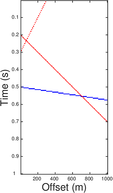
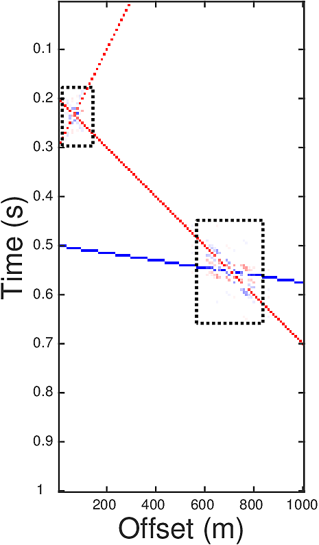
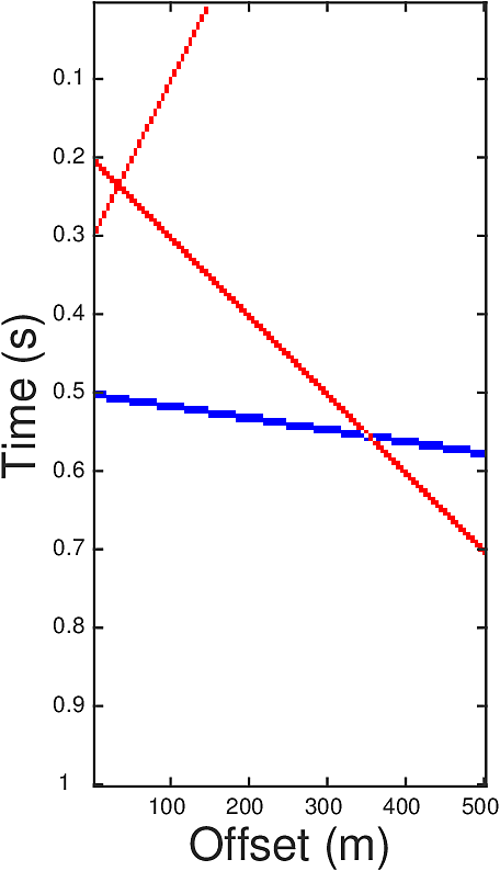
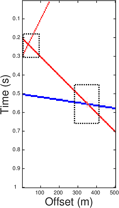
In order to utilize both the spatial similarity and the sparsity of \(G\) we proposed a TV norm regularizer that replaces the \(\ell_2\) norm in the definition of \(\mathcal{S}(\cdot)\) by an \(\ell_1\) norm and adds a vertical TV regularizer. The resulting problem is \[ \begin{equation} \begin{aligned} & G_{m,\textrm{est}}=\argmin\limits_{G_m} \|G_m\|_{TV}, \\ & \text{subject to} \ \ \hat{G}_m(\omega)=\hat{G}(\omega) \hat{f}(\omega)=\frac{\hat{d}(\omega)\hat{f}(\omega)}{\hat{q}(\omega)}, \omega\in \Omega, \end{aligned} \label{eqTV} \end{equation} \] where \(\|M\|_{TV}:=\sum\limits_{i,j} \|\nabla M(i,j))\|_{\ell_1}\) with \[ \begin{equation*} \begin{split} \nabla M(i,j) = \left[\begin{matrix}M(i,j)-M(i,j+1) \\ M(i,j)-M(i+1,j)\end{matrix}\right]. \end{split} \end{equation*} \] The low frequencies of \(G\) are obtained through the relation \[ \begin{equation*} \hat{G}(\omega) = \hat{G}_m(\omega)/\hat{f}(\omega), \omega \in \Omega_0. \end{equation*} \] Let us illustrate the effectiveness of our approach on a simple synthetic example. The ground truth \(G\) (Figure 1a) contains three events, each corresponding to a line in the reflectivity gather. Red dots in Figure 1a represent the value 1, blue are -1, and blanks are zeros. The crossing points of the events are those where \(\ell_1\) minimization (Equation \(\ref{eqL1}\)) has trouble to recover (Figure 1b). Here we have set \(\Omega=[30,50]\) and \(\Omega_0=[0,30]\). The auxiliary image \(G_m\) defined by \(G_m=f\ast G\) with parameter \(r=2\) is plotted in Figure 1c, where one can see the events are thickened. After performing the TV norm minimization, the inverted \(G_m\) in Figure 1d has much milder inaccuracy at the crossing points than that in Figure 1b.

Two comments are in order. A natural question is that whether we can increase spatial similarity by making the receivers denser. The answer is yes, but in doing so, we also increased the total number reflectivity series. In the end, the normalized error for each \(G_j\) is not decreased. Due to the limitation of space, we omit details of the argument.

The second comment is about the choice of \(r\). While mostly heuristic, we highlight some rough guidance. In principle, we want to choose \(r\) such that the derivative of the convolution kernel \(f\) are resolvable under \(\ell_1\) minimization. From the discussion in Candes and Fernandez-Granda (2014), the resolvability at least requires \(r \geq N/(T\omega_h)\) where \(\omega_h\) is the highest frequency in \(\Omega\), \(T\) is the sampling duration and \(N\) is the length of trace. On the other hand, we do not want \(r\) to be too large. Otherwise \(f\) becomes a powerful low-pass filter making the events in \(G_m\) lose resolution.

Acceleration

A typical seismic trace is sampled at 1,2,4 or 8 milliseconds time interval with a sampling duration about \(4-20\,\mathrm{s}\). This means that the trace length of a shot gather can be as long as 20000 samples. Performing the \(\ell_1\) or TV norm minimization, for example, on a \(20000\times 300\) shot gather can be quite expensive, especially if we want to raise one more dimension of \(G\) to include reflectivity series underlying a whole seismic line so as to obtain a 2 dimensional spatial continuation. As a consequence, it is desirable to use coarser time grid. Since the reflectivity series in \(G\) is assumed to be consist of spikes, which means it has a broad spectrum, then a downsampling may cause significant aliasing. On the other hand, our auxiliary variable \(G_m=f\ast G\) has relatively low energy in high frequency bands because the convolution kernel \(f\), besides delivering the already mentioned thickening benefit, also acts as a low-pass filter. This means traces corresponding to \(G_m\), i.e. \(d\ast f\), can be subsampled without much loss. The final extrapolation result is also barely affected because we only care about obtaining the low frequency information.

Numerical Experiments

We perform inversion experiments to demonstrate the effectiveness of extrapolation results of the proposed algorithm. We use the Marmousi model with about \(300\) meters water layer added on top of it to generate the data. Assuming that the data is only available in \(5-20\,\mathrm{Hz}\) frequency bands, which we generated using frequency domain finite difference modeling code. It is also reasonable to assume the availability of broadband (\(1-20\,\mathrm{Hz}\)) data for direct waves. Because we can easily obtain this data by doing forward modeling on a constant water velocity model. To perform extrapolation, we remove the direct waves from \(5-20\,\mathrm{Hz}\) synthetic data since they are too strong compared to the reflections and the refractions. We carry out the proposed algorithm twice to extrapolate from \(\Omega=\{5,5.1,5.2,...,20\}\,\mathrm{Hz}\) to \(\Omega_0=\{1,1.1,1.2,...,4.9\}\,\mathrm{Hz}\). First time on the reflectivity gathers (implemented in paralell for each shot)and the next time on the reflectivity series associated with a seismic line. We compare these two results. While implementing on a seismic line, we define the TV norm for all three directions (along time, sources, and receivers). The direct output of the extrapolation algorithm is \(\hat{G}(\omega),\omega \in \Omega_0\). We use it to construct the final extrapolated data by the formula \(\hat{d}(\omega)=\hat{G}(\omega)\hat{q}(\omega)+\hat{d}_0(\omega)\), where \(\hat{d}_0(\omega)\) is the data for direct waves at frequency \(\omega\) and \(\hat{q}(\omega)\) is the Fourier coefficient for the source wavelet. The inversion is performed using frequency continuation under inverse crime.

In the extrapolation algorithm, we set the time duration and the total number of samples in each reflectivity series to be \(10\,\mathrm{s}\) and \(400\) respectively (i.e. we take samples in every \(0.025\,\mathrm{s}\)) . We set the parameter \(r=10\) in the definition of \(f\), and solve the TV norm minimization problem (Eq \(\ref{eqTV}\)) approximately using the NESTA algorithm (Stephen Becker et al., 2011).

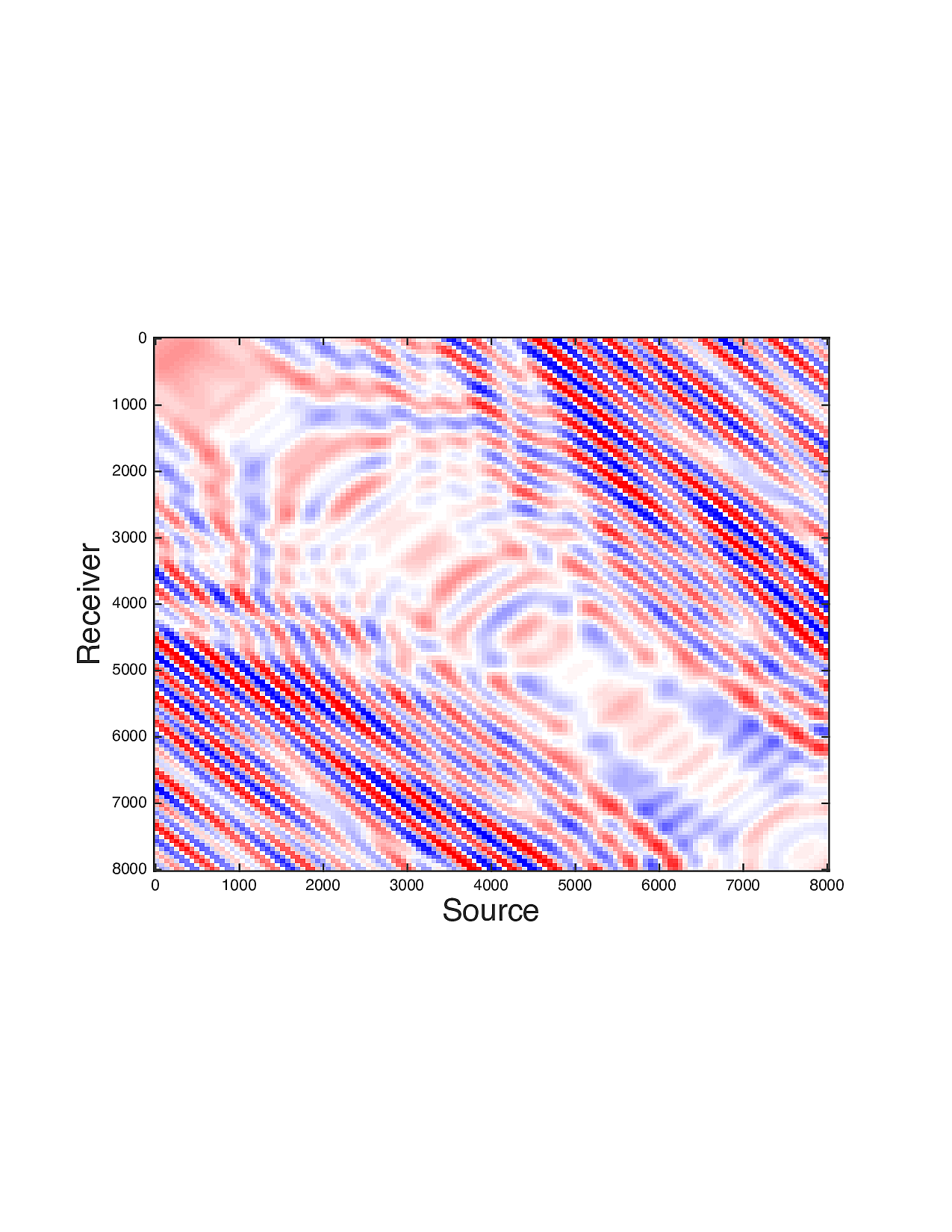
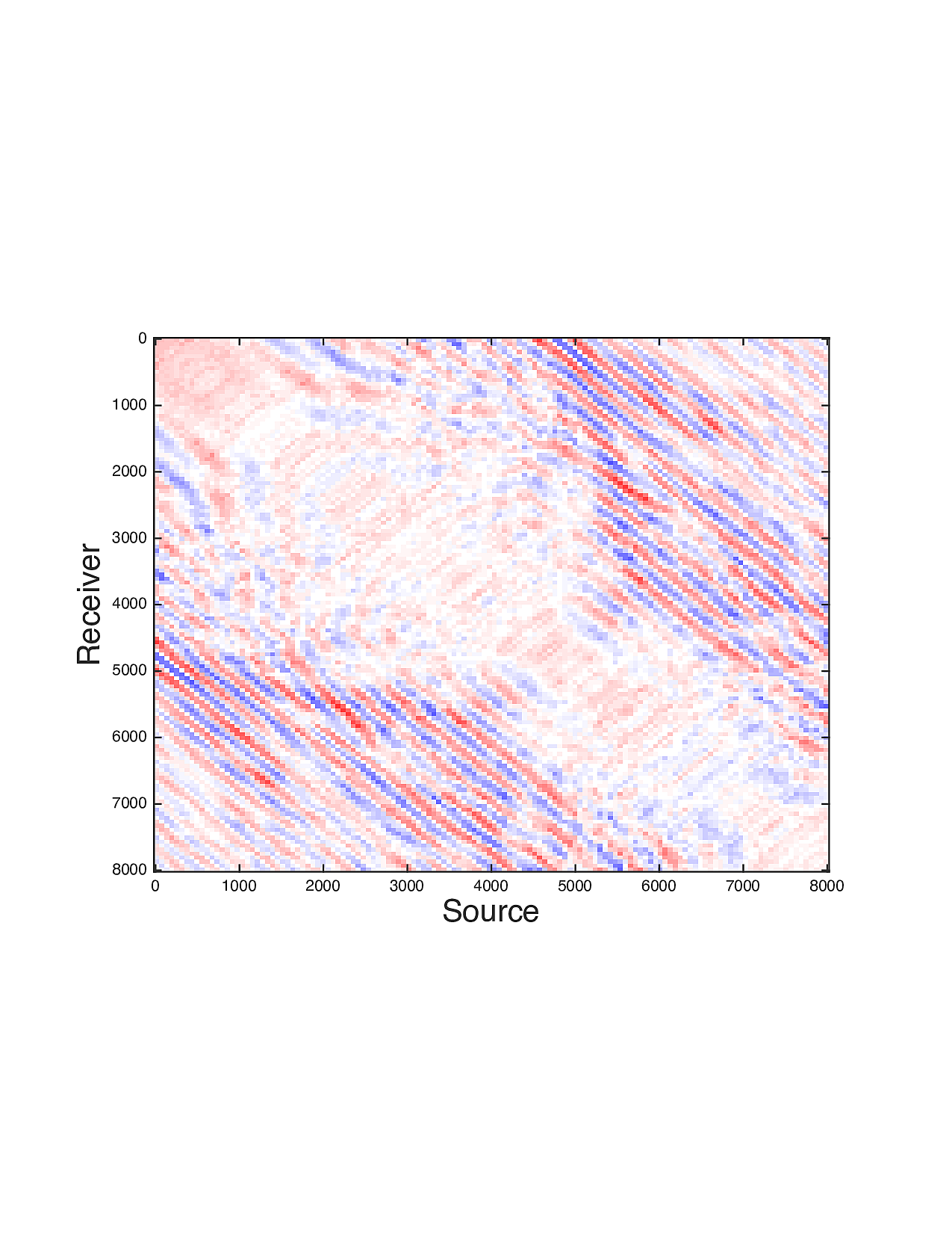
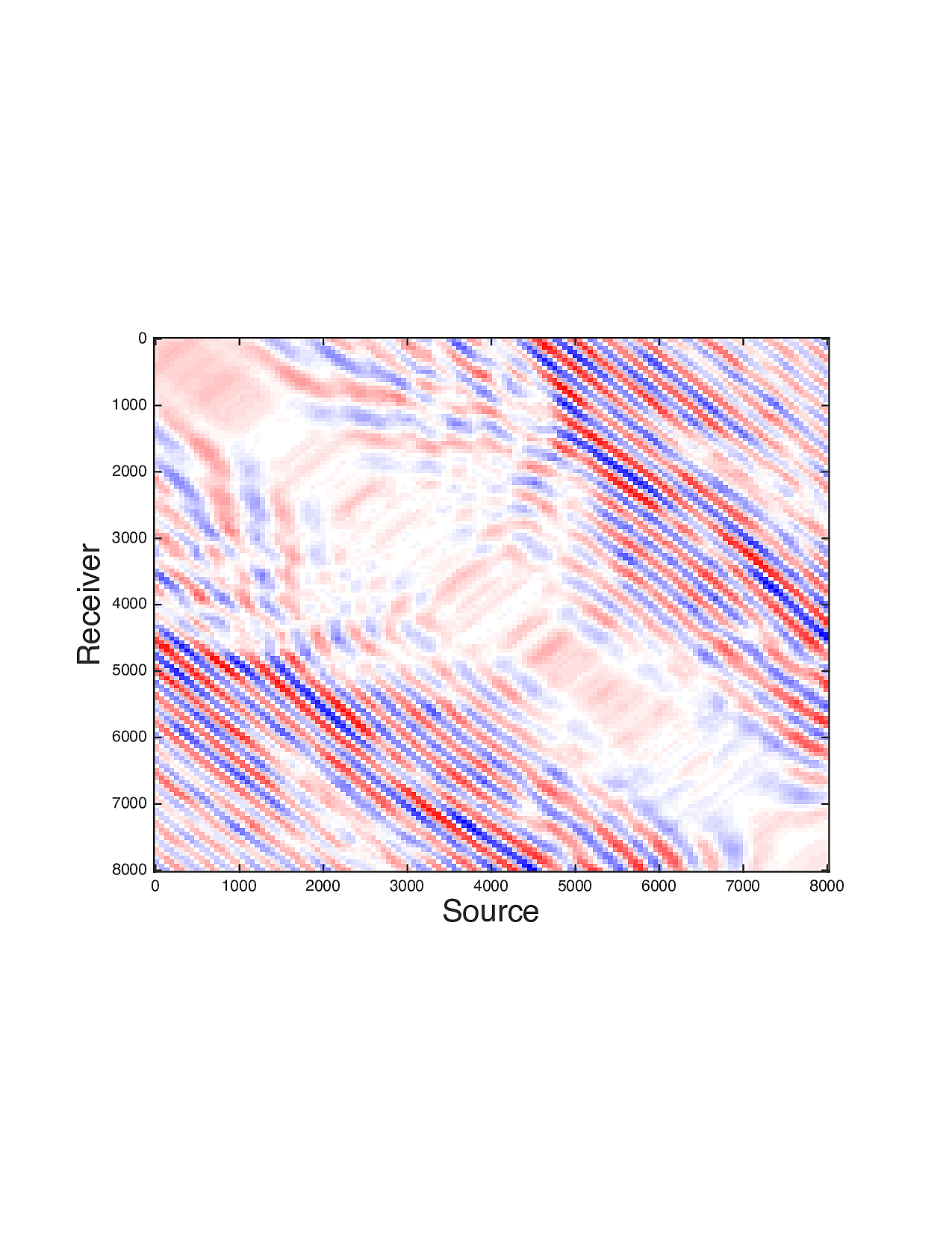
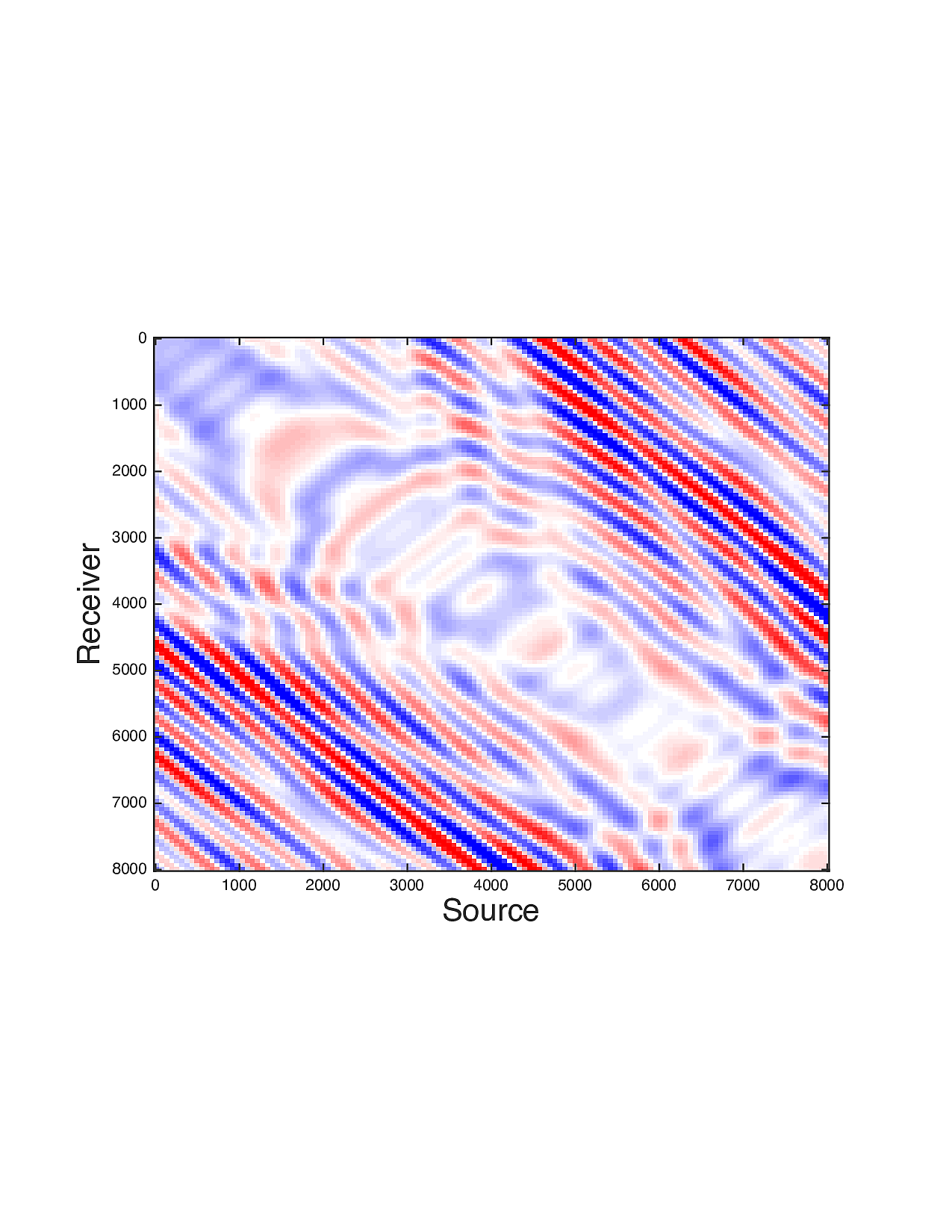
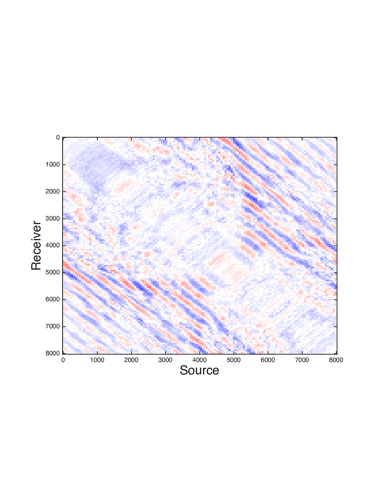
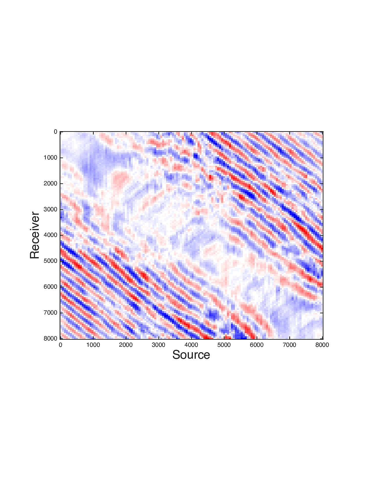
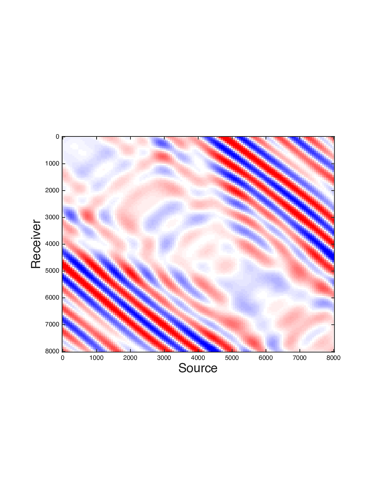
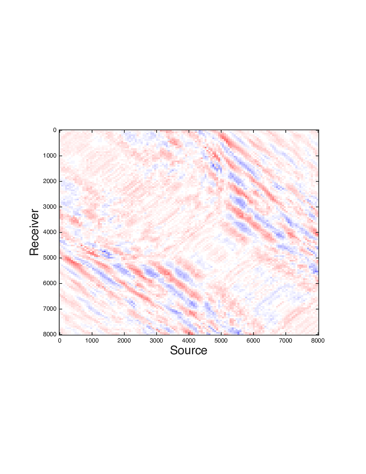
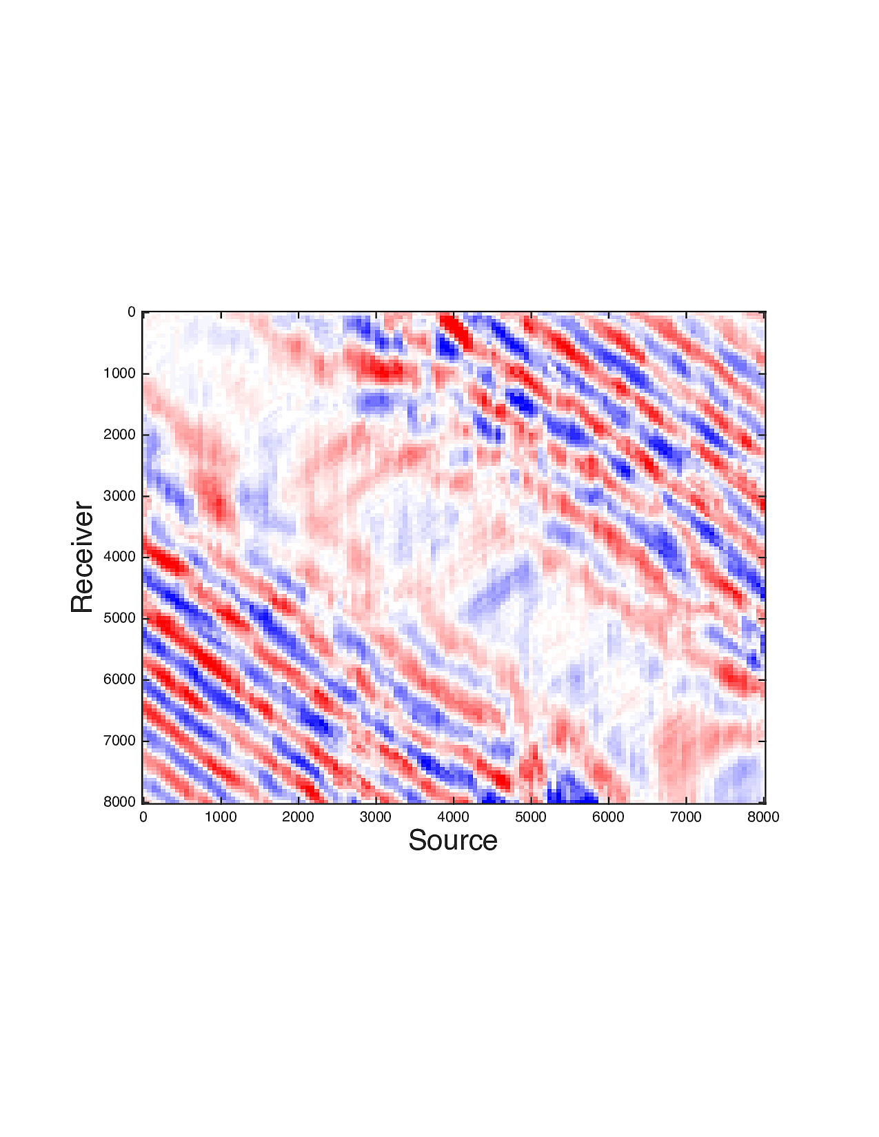
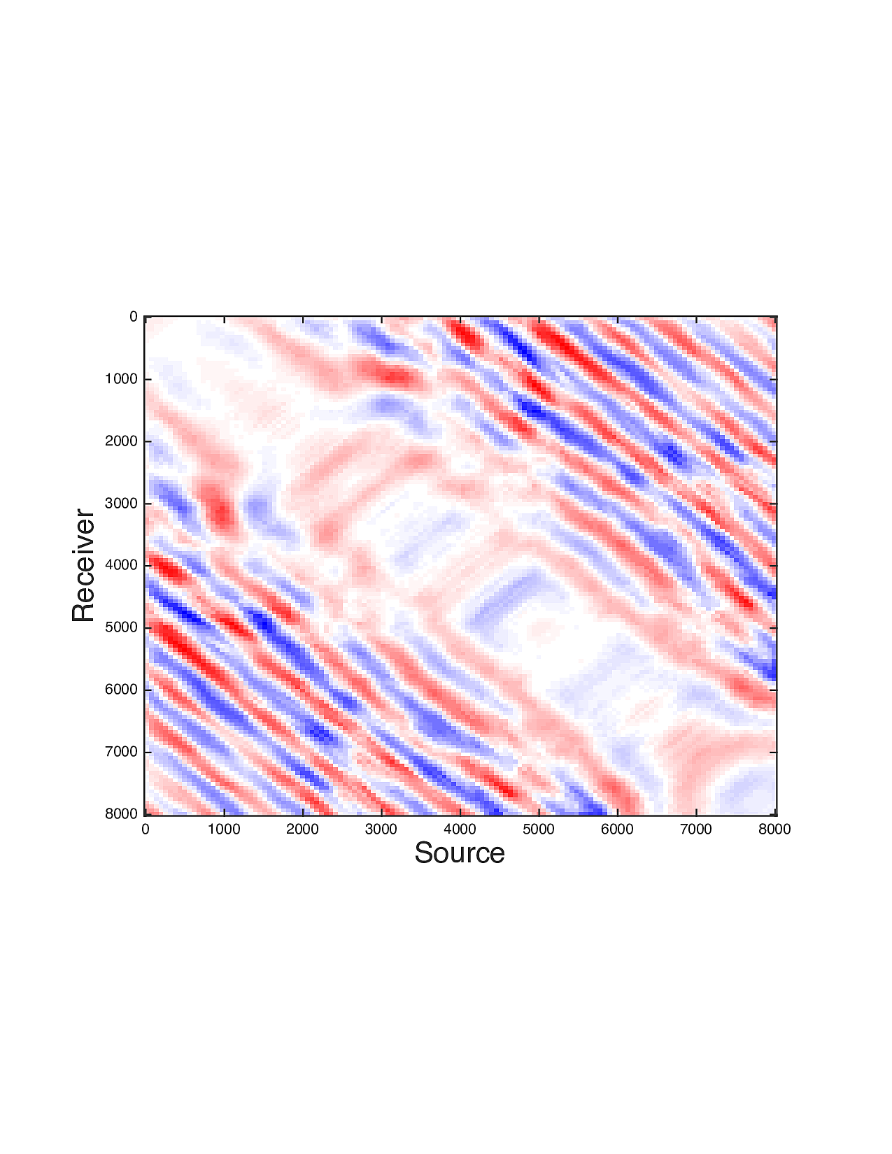
Figure 2 shows a comparison between the extrapolated data and the true data for three frequencies. Only the real part is plotted. Among the 12 sub-figures, the ones in the first column are frequency slices of the true data, those in the second column are extrapolated data with \(\ell_1\) minimization on reflectivity gathers, in the third column are extrapolated data with TV norm minimization on reflectivity gathers, and in last column are TV norm minimization on the seismic line. The first, second and third row corresponds to \(4\,\mathrm{Hz}\),\(3\,\mathrm{Hz}\) and \(2\,\mathrm{Hz}\) frequency slices, respectively. We can see that the use of spatial information has greatly enhanced and stabilized the result.

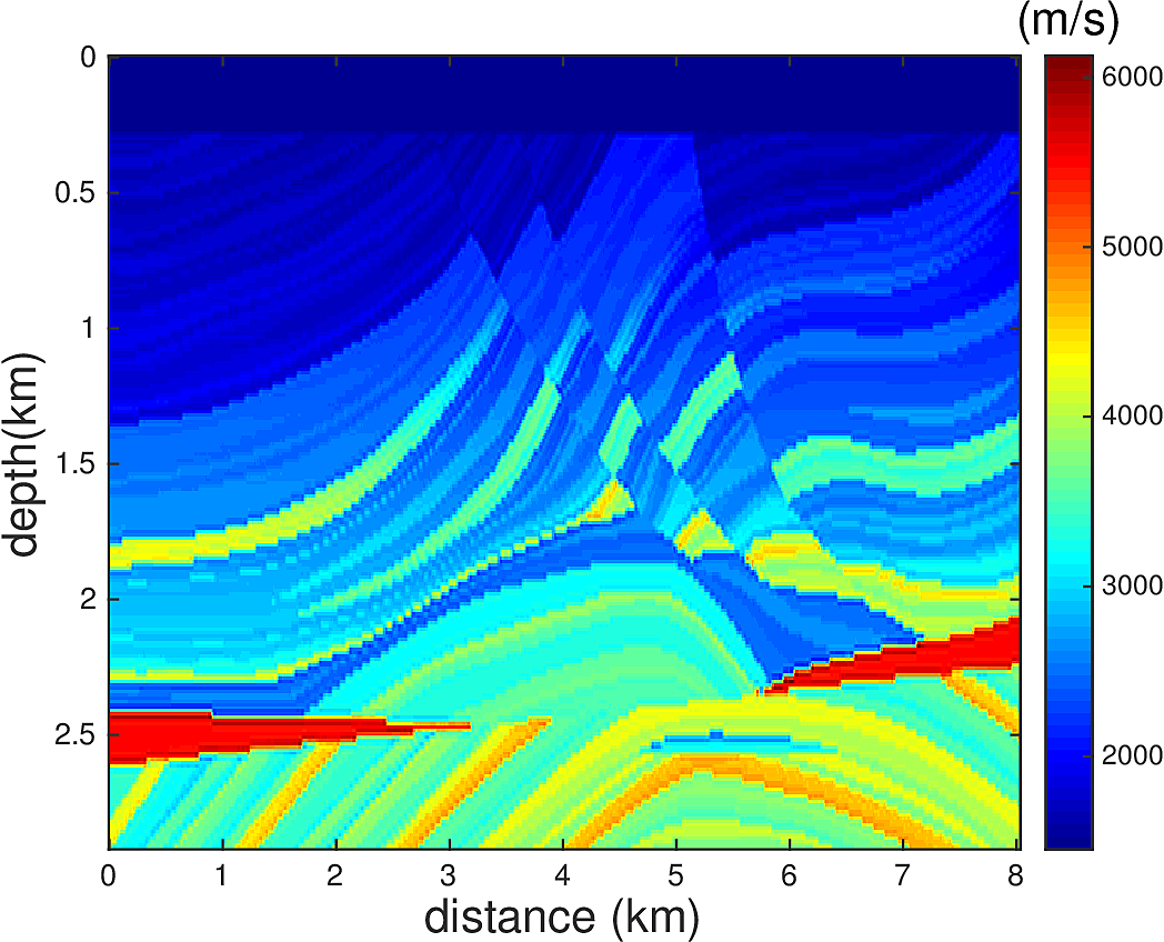
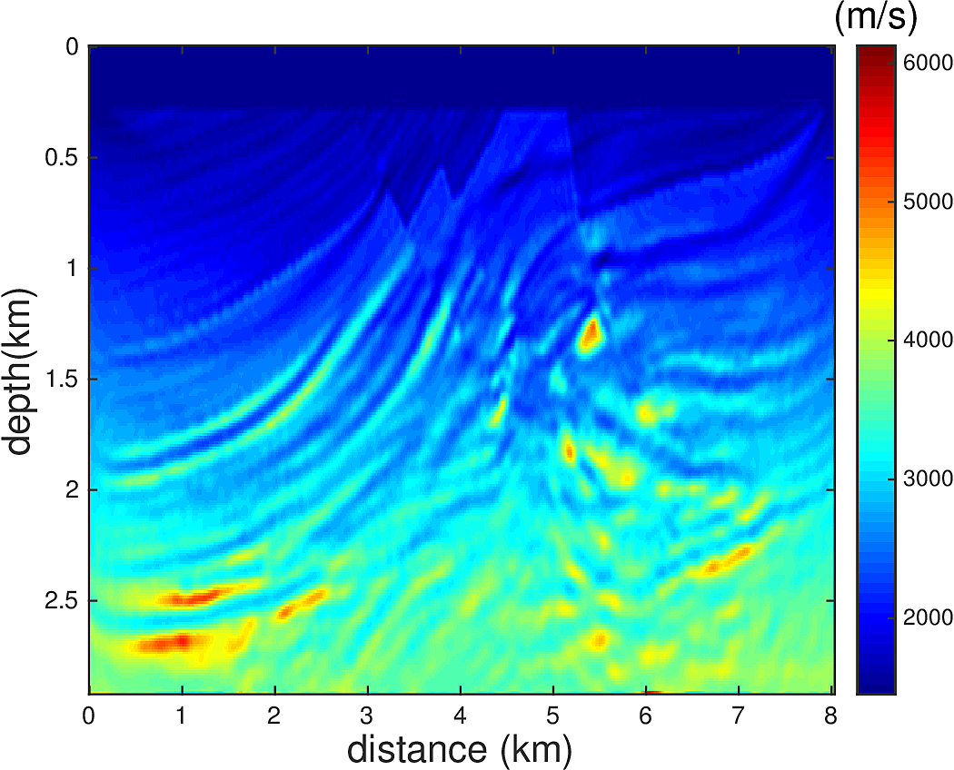
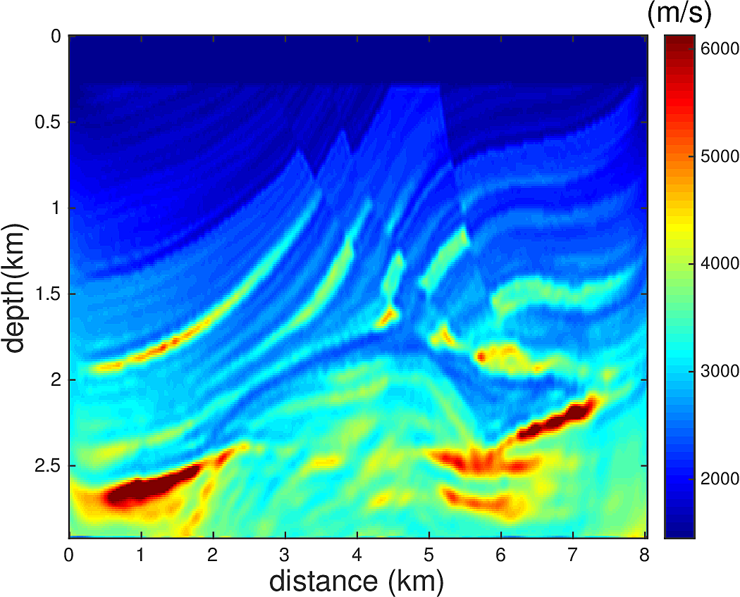
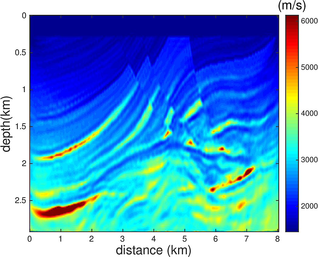
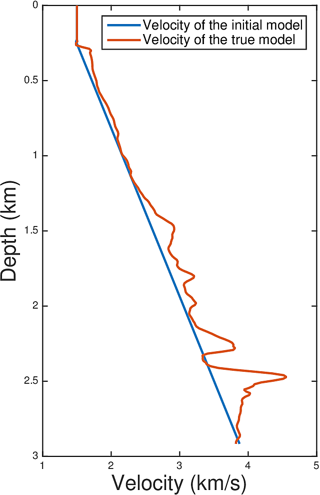
We perform Full Waveform Inversion using frequency continuation with overlapping frequency batches in the form of \(...,[5\,\mathrm{Hz},5.5\,\mathrm{Hz}],[5.5\,\mathrm{Hz},6\,\mathrm{Hz}],...\). For each frequency batch, we use \(20\) L-BFGS iterations. \(67\) uniformly spaced sources and \(134\) uniformly spaced receivers at depth of \(24\,\mathrm{m}\) from the top surface are used for this experiment. We do not allow water velocity above the sources and receivers to be updated, i.e., setting the gradient of each update to \(0\) for the grid points between \(0-24\,\mathrm{m}\) in depth. This is to make the inversion more robust to extrapolation errors. We use a 1D linear initial guess, whose velocity profile is plotted in Figure 4. Figure 3a shows the true velocity model. Figure 3b-d show the inversion results. Figure 3b shows the inverted model with narrowband \(5-15\,\mathrm{Hz}\) true data, 3c shows the inverted model with broadband \(1-15\,\mathrm{Hz}\) true data, and 3d shows the inverted model with \(1-5\,\mathrm{Hz}\) extrapolated data and 5-15Hz true data, where the extroplation is obtained by applying the proposed method to a seismic line. While the extrapolation is not entirely accurate, we demonstrated that if used carefully, it can help the FWI to correct large wavelength velocity errors in the initial model and accelerate the convergence.

Conclusion

In this paper, we proposed a method for low-frequency data extrapolation. The method inherits the stability of the traditional \(\ell_1\) minimization approach, while having both increased accuracy and speed. Synthetic inversion test shows that the artificial low frequency data is accurate enough to correct most of the large wavelength kinetic error in the initial model.

Although we assumed prior knowledge of the source wavelet throughout, the method can still fit seamlessly with existing source estimation procedures when the source is unknown. Specifically we need to add first a source estimation step before the extrapolation, which recovers the spectrum of \(q\) within \(\Omega\). After the extrapolated data is obtained, the subsequent inversion algorithm needs to have an embedded source estimation step (e.g., (Aleksandr Y. Aravkin et al., 2012)).

Acknowledgement

The authors would like to thank Xiang Li and Tristan van Leeuwen for useful discussions about the topic, and Curt Da Silva for sharing the 2D frequency modeling code. This work was financially supported in part by the Natural Sciences and Engineering Research Council of Canada Collaborative Research and Development Grant DNOISE II (CDRP J 375142-08). This research was carried out as part of the SINBAD II project with the support of the member organizations of the SINBAD Consortium.