Sparsity-promoting joint microseismic source collocation and source-time function estimation

Introduction

During hydraulic fracturing high-pressure fluid is injected through a well creating fractures in the rocks mainly containing shale (Montgomery and Smith, 2010). Shale contains oil traps but they are weakly connected due to the low permeability of shale. These fractures connect the oil traps, which ultimately enhances the oil productivity. In order to predict the production level of oil through these fracture induced reservoirs, it is extremely important to accurately map fracture propagation.

Hydraulic fracturing of rocks causes stress release, which eventually emits microseismic waves (Rutledge and Phillips, 2003). These waves carry important information about different source parameters such as source location, source origin time, source-time function etc. In microseismic imaging these induced seismic waves are recorded by surface receivers or receivers along a well. The resulting data is subsequently used to estimate different source parameters.

Traditional methods include travel time inversion, which relies on identification of different P and S components and traveltime picking of first arrivals of P and S components (Thurber and Engdahl, 2000; Waldhauser and Ellsworth, 2000). Identification of different components and traveltime picking of first arrivals is time consuming and can be extremely difficult in the presence of noise.

In recent years techniques have been developed that rely less or not at all on traveltime picking (Rentsch et al., 2007). Also the focus has shifted to the methods based on imaging (McMechan, 2010; Gajewski and Tessmer, 2005; Sun et al., 2015) and full-waveform inversion (FWI) (Sjögreen and Petersson, 2014; Kaderli et al., 2015). These methods rely less on first-arrival picking and are more robust to noise.

Kaderli et al. (2015) use FWI to invert for both the source-time function and source location. This method is based on estimating both parameters in an alternating fashion. However, the source location estimated by this method looks diffused and the estimated source-time function is noisier compared to the true wavelet.

Sun et al. (2015) use a hybrid imaging condition to produce high-resolution images of the source along both space and time axes. This method gives information on the source origin time but does not provide information on the source-time function itself.

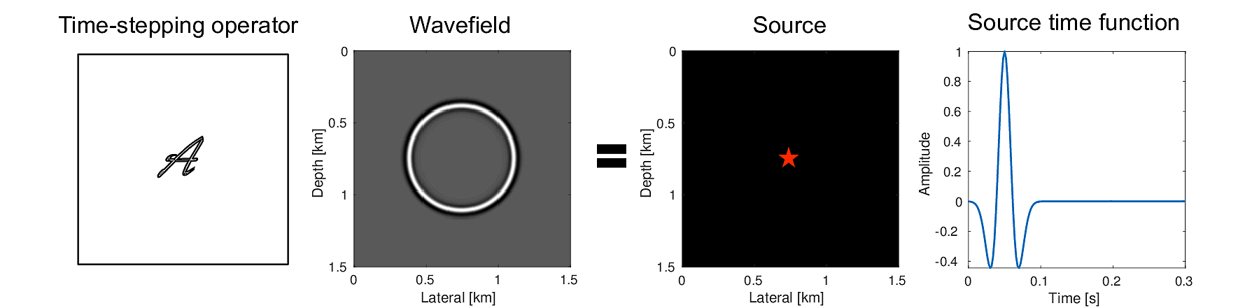
In this work, we propose a new method to simultaneously estimate both the source location and the source-time function. In particular, we aim to develop a method that requires only a smooth background velocity model and is robust in the presence of noise. Our approach is based on the co-sparsity property (Nam et al., 2013) of the physics of waves. Co-sparsity of a signal \(\vector{u}\) corresponds to the property that there exist a so-called analysis operator \(\boldsymbol{\Omega}\) that maps \(\vector{u}\) to a vector \(\vector{z}\) with few non-zero coefficients. In the context of waves, the finite-difference modelling operator acts as an analysis operator for wavefields. This implies that wavefields under the action of a finite-difference modelling kernel can be focused to sources generating these wavefields (Figure 1). We exploit this property of wavefields to locate microseismic events and estimate the source time function jointly. To arrive at a computational feasible scheme, we use the Linearized Bregman (LBR) algorithm (Yin et al., 2008; Lorenz et al., 2014; Herrmann et al., 2015) to solve the above mentioned problem.

Methodology

FWI based methods aim to solve \[ \begin{equation} \minim_{\vector{f}\in\R^{n_x},\,\vector{w}\in\R^{n_t}} \quad \|\mathcal{F}(\vector{m})\vector{f}\vector{w}^T - \vector{d}\|, \label{eq:master} \end{equation} \] where \(\mathcal{F}(\vector{m})=\mathcal{P}{\mathcal{A(\vector{m})}}^{-1}\) is the forward modeling operator and \(\{\vector{f},\,\vector{w}\}\) represent the pair of unknowns, namely the spatial component of the source \(\vector{f}\in\R^{n_x}\), with \(n_x\) the size of the spatial grid, and source-time signature \(\vector{w}\in\R^{n_t}\) with \(n_t\) the number of time samples. The linear operator \(\mathcal{P}\) restricts wavefields to the receiver locations, followed by a vectorization. \({\mathcal{A(\vector{m})}}\) implements a time-stepping finite-difference modelling operator, parameterized by the background squared slowness \({\vector{m}}\). The vector \(\vector{d}\) contains the set of microseismic measurements recorded at receivers either located at the surface or along a well or both. In this formulation, the spatial and time components of the source appear separable via the outer product \(\vector{f}\vector{w}^T\) with \(^T\) denoting the transpose. This special structure allows Kaderli et al. (2015) to treat the spatial and temporal components of the source separately and estimate them in an alternating fashion. The obvious limitation of this approach is that it can not estimate both unknown vectors simultaneously and another limitation is that it can only work when multiple sources have the same signature. This method can be extended for multiple source cases by using a separable higher rank approximation, where the rank will be equal to the number of sources. Another obvious limitation of this extended method is that we need prior information about the number of sources.

Instead of using the separable rank-one or higher rank approximation, we use a lifting technique that is linear for a single matrix \(\vector{Q}\), which contains the spatial-temporal distribution for different sources—i.e. the \((i,j)\) entry in \(\vector{Q}_{i,j} = {q}(x_i,t_j)\). Although it can become expensive to handle such a big matrix instead of handling the two vectors \((\vector{f}\) and \(\vector{w})\), it gives us more flexibility to simultaneously estimate both the source location and the source-time signature for multiple sources with different source signatures without having any prior assumption on the number of sources.

Kitić et al. (2016) used the fact that the wave equation is in itself an excellent sparsity-promoting transform to locate the coordinate of sound sources based on microphone recordings. We used similar approach in realistic seismic settings to jointly estimate the microseismic source-location and time-signature. For a given spatio-temporal wavefield \(\vector{U}\) (generated by applying the inverse of the \({\mathcal{A(\vector{m})}}\) on a sparse source \(\vector{Q}\)), the action of wave equation on this wavefield, i.e., \({\mathcal{A(\vector{m})}}{\vector{U}}= {\vector{Q}}\), acts as a sparsity-promoting transform. For a sufficiently accurate velocity model, the wave equation maps the full wavefield, \(\vector{U}\), to a spatially focused source \(\vector{Q}\) (Figure 1). Hence, for point sources the finite-difference operator \(\mathcal{A(\vector{m})}\) acts as a sparsity-promoting transform in space when \(\vector{Q}\) contains a few point sources. By assuming sources to be localized in space and smooth along time, we solve \[ \begin{equation} \minim_{\vector{U}} \quad \|\mathcal{A(\vector{m})}\vector{U}\|_{1,2} \quad \text{subject to} \quad \|\mathcal{P}\vector{U} - \vector{d}\|_2 \leq \epsilon \label{eqMoti} \end{equation} \] with \(\epsilon\) is the two-norm of the noise. By solving this minimization problem, we find a wavefield \(\vector{U}\) that has the smallest \(\ell_1\)-norm in space and smallest \(\ell_2\)-norm in time (denoted by the norm \(\|\cdot\|_{1,2})\)) when acted upon by the wave equations while fitting the data to within \(\epsilon\). From the inverted wavefield, both the location of the sources and source-time signatures can readily be extracted.

To make the above optimization problem (equation \(\ref{eqBPDN}\)) more tractable, we invoke a change of variables \(\vector{Q} = \mathcal{A(\vector{m})}\vector{U}\) so we arrive at \[ \begin{equation} \minim_{\vector{Q}} \quad \|\vector{Q}\|_{1,2} \quad \text{subject to}\quad\|\mathcal{F}(\vector{m})\vector{Q} - \vector{d}\|_2 \leq \epsilon. \label{eqBPDN} \end{equation} \] For a given \(\vector{m}\), Equation \(\ref{eqBPDN}\) takes the form of the classic Basis Pursuit Denoising(BPDN) Problem.

Motivated by recent successful application of the linearized Bregman (Yin et al., 2008; Lorenz et al., 2014) to least-squares migration (Herrmann et al., 2015), we relax the \(\|.\|_{1,2}\) norm to a mixed \(\|.\|_{1,2}\) and Frobenius norm—i.e., we solve \[ \begin{equation} \minim_{\vector{Q}} \quad {\lambda}\|\vector{Q}\|_{1,2} + \frac{1}{2}\|\vector{Q}\|_F^2 \quad \text{s.t.}\quad \|\vector{\mathcal{F}(\vector{m})} \vector{Q} - \vector{d}\|_2 \leq \epsilon. \label{eqSrcest} \end{equation} \] As in regular linearized Bregman, the parameter \(\lambda\) controls the trade of between the “sparsity” and regular two-norm terms. When \(\lambda\uparrow\infty\) the solution of Equation \(\ref{eqSrcest}\) approaches the solution of Equation \(\ref{eqBPDN}\). Compared to BP, Equation \(\ref{eqSrcest}\) permits a relatively simple iterative algorithm (See Algoritm 1 below), which is robust to noise.

In Algorithm 1, the dynamic step length \({t}_{k}\) according to Lorenz et al. (2014) is given by \[ \begin{equation*} {t}_{k} = \frac{\|\mathcal{F}(\vector{m}) \vector{Q}_{k} - \vector{d}\|^2}{\|\mathcal{F}(\vector{m})^T(\mathcal{F}(\vector{m})\vector{Q}_{k} - \vector{d})\|^2}. \end{equation*} \] The operator \(\mathrm{Prox}_{\lambda}\|.\|_{1,2}({c}):= \argmin_t {\lambda}\|{b}\|_{1,2} + \frac{1}{2}\|{c}-{b}\|_F^2\) is the proximal mapping (Combettes and Pesquet, 2011) of the \(\ell_{12}\) norm with \(\Pi_\epsilon (\vector{x}) = \mathrm{max} \{{0,1-\frac{\epsilon}{\|\vector{x}\|}}\}.(\vector{x})\) the projection on to \(\ell_2\)-norm ball.

Compared to other sparsity-promoting approaches, this algorithm is relatively simple to implement and has very few tuning parameters.

Line 2 in Algorithm 1 corresponds to a projection of the residual, given by forward modeling with the current estimate for \(\vector{Q}\) on the \(\ell_2\)-norm ball of size \(\epsilon\), followed by injection of this scaled residual into the grid and time-stepping backwards in time with the adjoint of the wave equation. The result \(\vector{V}\) of this is used to update \(\vector{Z}\), the auxiliary variable in line 3. To focus the resulting estimate for the source wavefield, we apply the proximal operator that sparsifies \(\vector{Q}\) along the spatial coordinates and that keeps the energy along time in check.

After solving for \(\vector{Q}\), we obtain a final image of the locations of the microseismic events by performing a summation of absolute amplitude of the estimated \(\vector{Q}\) along time at each grid point. This results in an intensity plot where the source locations appear as outliers. We obtain estimates for the time-signature by extracting the temporal variations of the estimated wavefield at the spatial locations of the maxima in the intensity (Figure 1).

Numerical Experiments

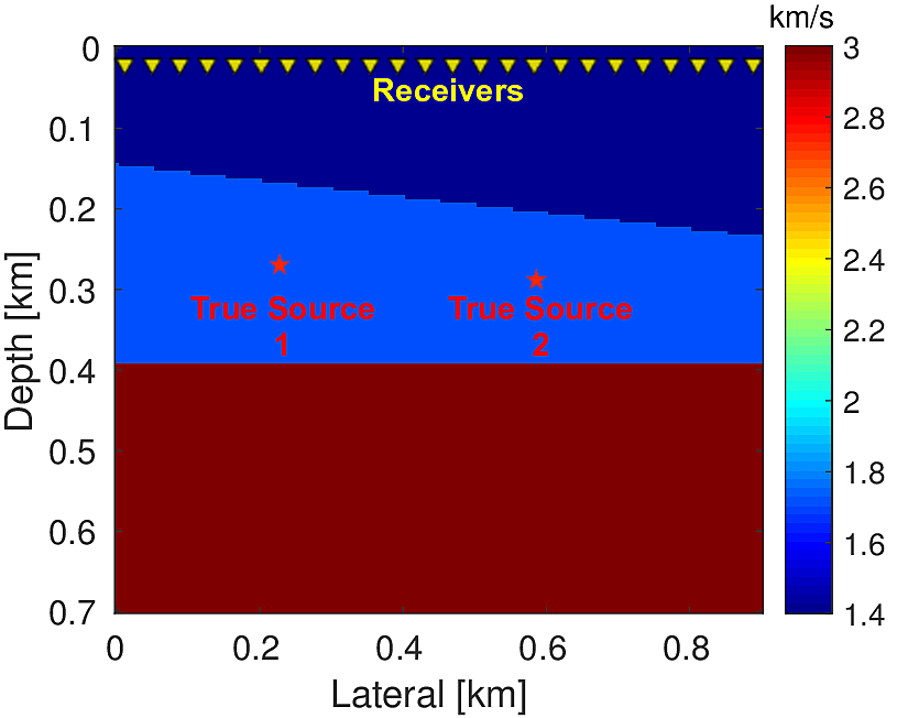
We performed two different experiments in order to demonstrate the ability of proposed algorithm. For both the experiments we used \(3\) layered synthetic velocity model of dimension \(0.9\,\mathrm{km} \times 0.7\,\mathrm{km}\) (\(181 \times 141\) points) (Figure 2a & 4a). We used time-stepping finite-difference modelling method to generate microseismic data. For both the experiments we used receivers at \(20.0\, \mathrm{m}\) depth from the top surface and separated by \(10.0\, \mathrm{m}\) (Figure 2a & 4a) to record the data. For all these experiments we assume that both the source location and source time function are unknown.

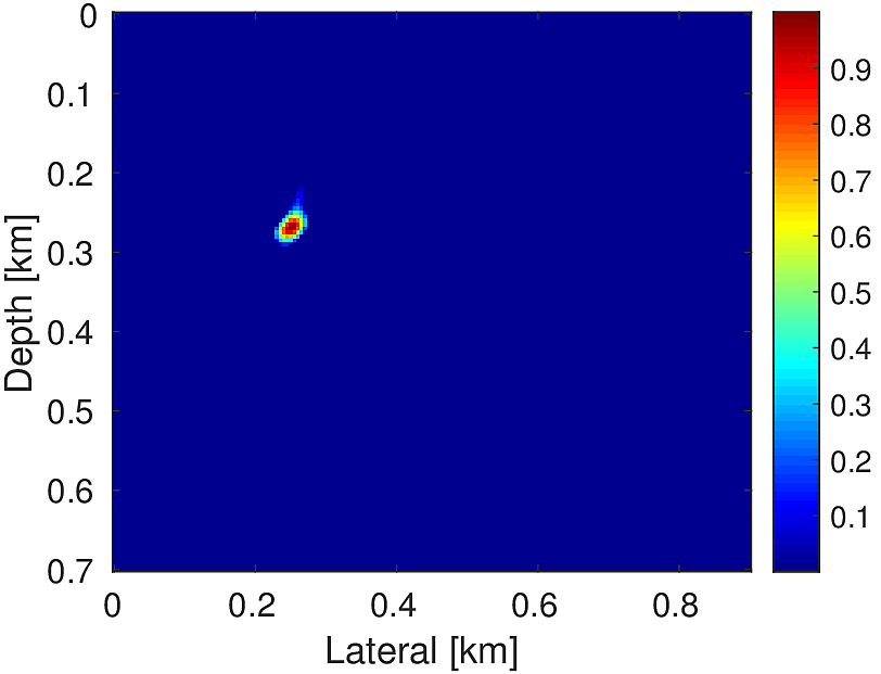
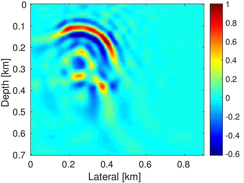
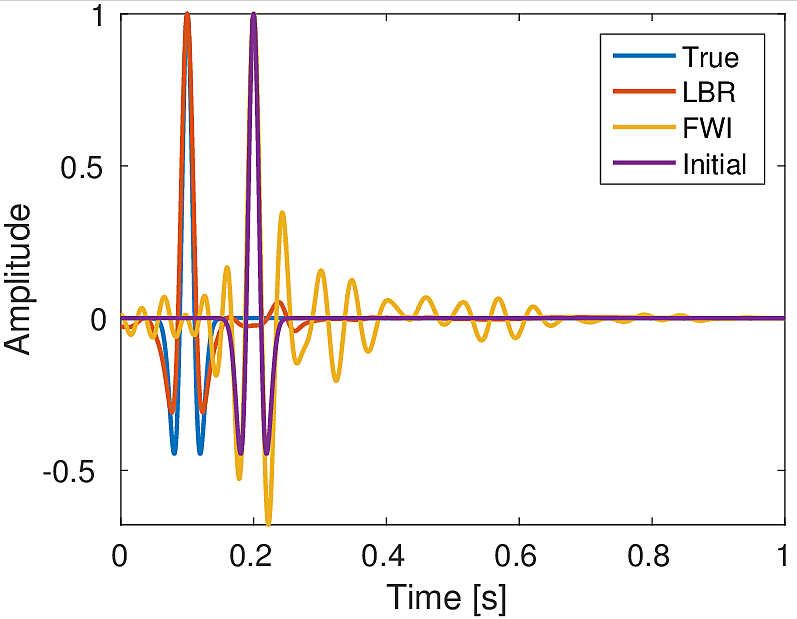
Experiment 1—True velocity experiment

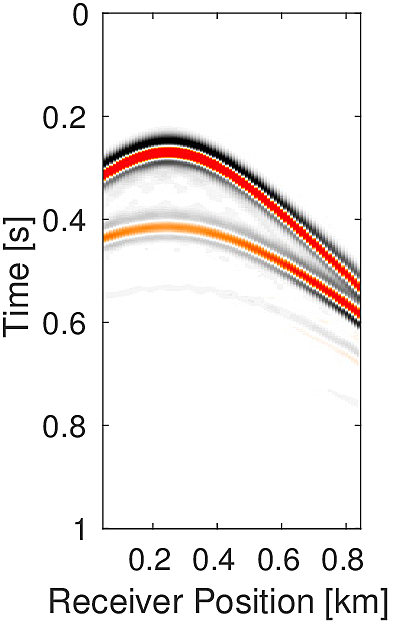
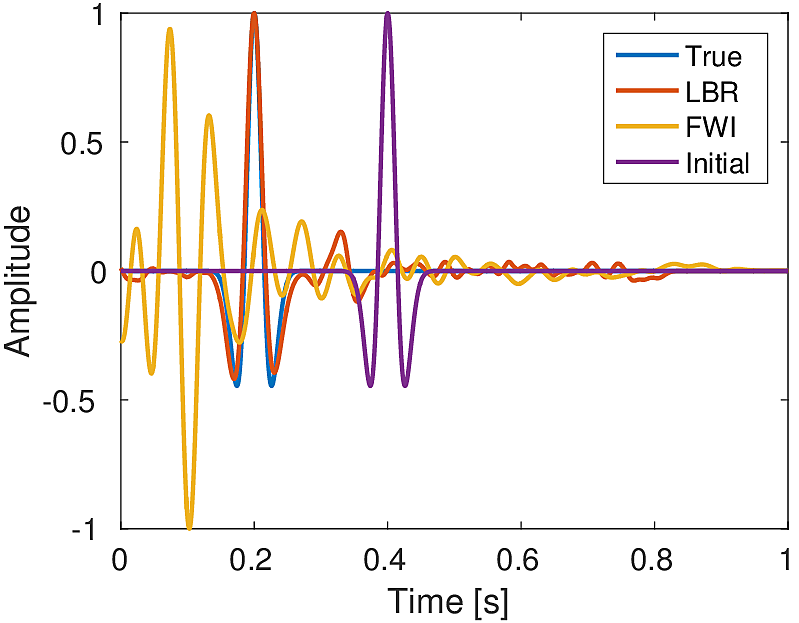
In the first experiment, we estimate the source location and source-time function using noise-free synthetic microseismic measurements. Here, we assume that we know the true velocity. We use a single source located at (\(0.25\, \mathrm{km}\) , \(0.27\, \mathrm{km}\)) (Figure 2a) with Ricker wavelet of peak frequency \(20.0\, \mathrm{Hz}\) to generate data (Figure 3) of record length \(1.0\, \mathrm{s}\). We compare our method with the FWI based (Kaderli et al., 2015) method. We assume that both the source location and the source-time function are unknown. We performed \(20\) iterations each of Linearized Bregman (LBR) and FWI with \(4\) inner iterations for each of unknown source location and unknown source wavelet in case of FWI. Starting with zero initial guess our method gives a focused source location (Figure 2b) in comparison to the FWI-based method (Figure 2c). Moreover, our method is able to give a good estimation of the source-time function (Figure 2d) in comparison to FWI, which looks noisier and shifted in comparison to the true wavelet. For the FWI-based method, we started with an initial guess of source wavelet as Ricker wavelet of \(20.0\, \mathrm{Hz}\) (centred at \(0.2\, \mathrm{s}\)).

Experiment 2—Smooth background velocity and noisy data experiment

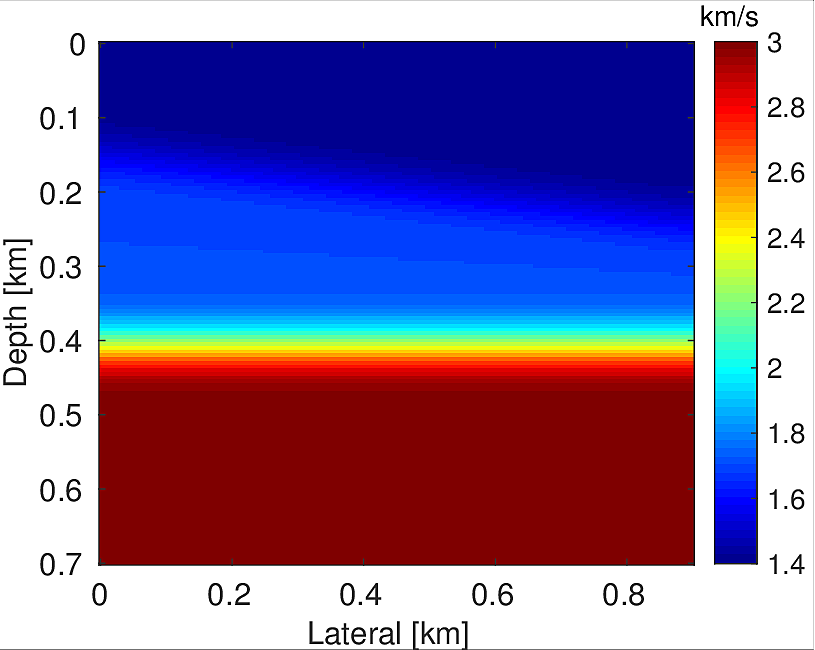
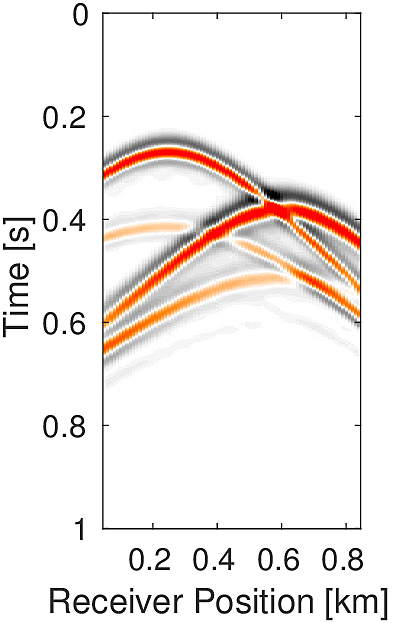
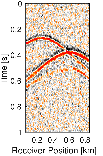
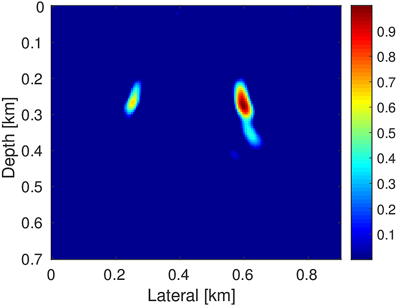
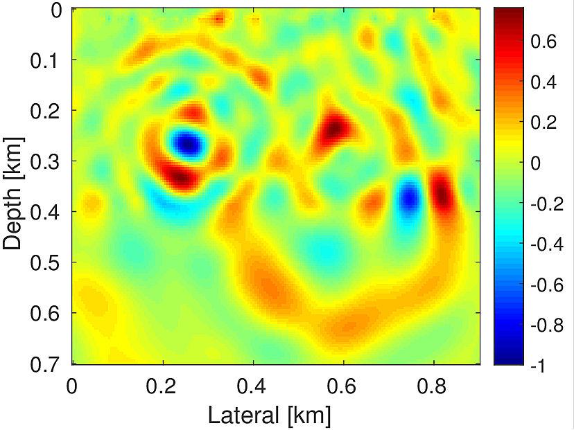
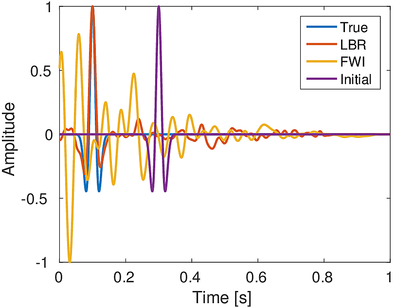
In practice, we generally do not have a detailed velocity model. At most we have a smooth background-velocity model available. Assuming that we only have access to a smooth background-velocity model (Figure 4b), we perform this experiment. We also assume that our data is noisy. We use two sources located at (\(0.25\, \mathrm{km}\) , \(0.27\, \mathrm{km}\)) and (\(0.60\, \mathrm{km}\) , \(0.28\, \mathrm{km}\)) (Figure 4a) and source wavelet as Ricker wavelet with peak frequency of \(20.0\, \mathrm{Hz}\) (centered at \(0.1\, \mathrm{s}\)) and \(15.0\, \mathrm{Hz}\) (centered at \(0.2\, \mathrm{s}\)), respectively to generate data (Figure 5a) of record length \(1.0\, \mathrm{s}\). We add to it low frequency (up to \(45.0\, \mathrm{Hz}\)) random noise to get the noisy data (Figure 5b) (SNR = \(0.34\)). We use noisy data and smooth velocity to jointly estimate the source location and source time function for both sources. We perform \(150\) iterations each of Linearized Bregman and FWI with \(4\) inner iterations each for inverting for the source location and source-time function. For FWI, we use a separable rank \(2\) matrix (Equation \(\ref{eq:rank2}\)). Here we aim to solve following rank \(2\) system: \[ \begin{equation} \minim_{\vector{f_1},\vector{f_2}\in\R^{n_x},\,\vector{w_1},\vector{w_2}\in\R^{n_t}} \quad \|\mathcal{F}(\vector{m})(\vector{f_1}\vector{w_1}^T + \vector{f_2}\vector{w_2}^T) - \vector{d}\|, \label{eq:rank2} \end{equation} \] In order to decide the rank, we assume in this case that we know the number of sources a priori. Conversely, for our method, we do not need to know the number of sources a priori. With zero initial guess our method is able to give a good estimation of the location of both the sources (Figure 6a) in comparison to the FWI based method (Figure 6b). Also our method is able to give a good approximation of the true source-time function at both the locations in comparison to FWI (Figures 6c & 6d). For the FWI-based method, we started with an initial guess of the source wavelets \(\vector{w_1}\) and \(\vector{w_2}\) as Ricker wavelet with peak frequency of \(20.0\, \mathrm{Hz}\) (centered at \(0.3\, \mathrm{s}\)) and \(15.0\, \mathrm{Hz}\) (centered at \(0.4\, \mathrm{s}\)), respectively.

Conclusions

We have presented a new methodology to simultaneously locate microseismic events and estimate the source-time functions from surface microseismic measurements. We exploited the underlying physics of wave propagation by focusing the microseismic measurements back to its true source location. Linearized Bregman based method seems to be robust to noise and simple to be implemented with very few tuning parameters. It is also able to jointly invert for the source location and source-time function without any prior knowledge of these parameters. We demonstrated that starting with zero initial guess, even when data is noisy and we only have a smooth background velocity model available, we are able to recover accurate approximations of both the source locations and source-time functions. We also demonstrated the success of our method when we have microseismic sources with different signature.

Acknowledgement

We would like to acknowledge Mathias Louboutin for sharing the time stepping finite difference modeling code. This work was financially supported in part by the Natural Sciences and Engineering Research Council of Canada Collaborative Research and Development Grant DNOISE II (CDRP J 375142-08). This research was carried out as part of the SINBAD II project with the support of the member organizations of the SINBAD Consortium.