Uncertainty quantification for Wavefield Reconstruction Inversion using a PDE free semidefinite Hessian and randomize-then-optimize method

The data of full-waveform inversion often contains noise, which induces uncertainties in the inversion results. Ideally, one would like to run a number of independent inversions with different realizations of the noise and assess model-side uncertainties from the resulting models, however this is not feasible because we collect the data only once. To circumvent this restriction, various sampling schemes have been devised to generate an ensemble of models that fit the data to within the noise level. Such sampling schemes typically involve running multiple inversions or evaluating the Hessian of the cost function, both of which are computationally expensive. In this work, we propose a new method to quantify uncertainties based on a novel formulation of the full-waveform inversion problem – wavefield reconstruction inversion. Based on this formulation, we formulate a semidefinite approximation of the corresponding Hessian matrix. By precomputing certain quantities, we are able to apply this Hessian to given input vectors without additional solutions of the underlying partial differential equations. To generate a sample, we solve an auxiliary stochastic optimization problem involving this Hessian. The result is a computationally feasible method that, with little overhead, can generate as many samples as required at small additional cost. We test our method on the synthetic BG Compass model and compare the results to a direct-sampling approach. The results show the feasibility of applying our method to computing statistical quantities such as the mean and standard deviation in the context of wavefield reconstruction inversion.

Introduction

Full-waveform inversion (FWI) aims to reconstruct the Earth’s subsurface velocity structure from data measured at the surface (Tarantola and Valette, 1982a; Virieux and Operto, 2009). The measured data of FWI often contains noise that leads to uncertainties in data. As a result of fitting this noisy data, these uncertainties propagate through the inversion procedure, which result in uncertainties in the final model (Malinverno and Briggs, 2004). The conventional approach to study these random fluctuations is to use the Bayesian inference approach to formulate the posterior distribution of the unknown parameter and generate, say, mean and standard deviation plots (Kaipio and Somersalo, 2004). Unfortunately the FWI is a strongly non-linear inverse problem and the forward problem of FWI is computationally expensive, which leads to difficulties in the explicit computation of the parameter space distribution and in calculating the mean and pointwise variance of velocity (Tarantola and Valette, 1982b).

Wavefield reconstruction inversion (WRI) (Leeuwen and Herrmann, 2013; Peters et al., 2014) is a new approach to solve wave-equation based inversion problems. Unlike conventional FWI, which at each iteration solves the wave-equation exactly, WRI considers the wave-equation as a \(\ell_2\)-norm penalty term in the objective function, weighted by a penalty parameter. For WRI, when either the velocity or the wavefield is fixed, the problem becomes a linear fitting problem in the other variable. As a result, WRI is “less non-linear” compared to FWI. Additionally, the WRI enjoys an approximate diagonal Hessian of the objective function that does not require additional partial-differential equation (PDE) solves (Leeuwen and Herrmann, 2013). Given these advantages of WRI, Fang et al. (2015) proposed a posterior distribution based on WRI and produced samples with an Gaussian distribution based on the diagonal approximation of the Hessian.

The diagonal approximation of the Hessian utilized by Fang et al. (2015) does not account for the statistical correlations of the wavefields with the model vectors, resulting in a poor approximation of the probability density when the penalty parameter is large. In this work, we propose to use a more accurate semidefinite Hessian approximation (Leeuwen and Herrmann, 2015) to approximate the posterior distribution. This Hessian does involve additional PDE-solves, but the necessary wavefields can be easily precomputed and stored for later use. Thus, we can still apply the Hessian to given input vectors at little additional computational cost.

The conventional approach to draw samples from a Gaussian distribution consists of two steps: (1) minimize the negative logarithm function of the posterior distribution to obtain the maximum a posteriori (MAP) estimate, i.e., the point that maximizes the posterior probability; (2) compute the Cholesky factor of the covariance matrix at the MAP estimate and use it to draw samples (Martin et al., 2012). In practice, the latter step requires us to form the full Hessian matrix explicitly and is computationally expensive (Rue, 2001). In this work, we utilize the so-called randomize-then-optimize (RTO) method (Solonen et al., 2014), which generates a sample from a Gaussian distribution by solving a stochastic least-squares problem involving the covariance matrix. By using our PDE-free Hessian, we can solve these least-squares problems efficiently using standard solvers such as CGLS or LSQR (Paige and Saunders, 1982). This results in a scalable algorithm for generating samples from the posterior distribution.

Posterior Distribution for WRI

Tarantola and Valette (1982b) first introduced the Bayesian approach to the seismic inverse problem and proposed the general framework of statistical FWI. Based on the Bayes’ law, for a model parameter \(\mvec\) with \(n_{\text{grid}}\) points, the posterior distribution \(\rhopost(\mvec|\dvec)\) of \(\mvec\) given data \(\dvec\) consisting \(n_{\text{src}}\) shots and \(n_{\text{freq}}\) frequencies is proportional to the product of the likelihood distribution \(\rholike(\dvec|\mvec)\) and the prior distribution \(\rhoprior(\mvec)\) yielding: \[ \begin{equation} \rhopost(\mvec|\dvec) \propto \rholike(\dvec|\mvec) \rhoprior(\mvec). \label{Bayes} \end{equation} \] In other words, the most probable model vectors \(\mvec\) that correspond to our data \(\dvec\) are those that likely correspond to our prior beliefs about the underlying model, irrespective of data, (i.e.,\(\rhoprior(\mvec)\)) as well as those that generate data \(\dvec\) that are probabilistically consistent with our underlying physical and noise model (i.e., \(\rholike(\dvec|\mvec)\)). This formulation allows us to explicitly write down expressions for the last two terms, while simultaneously ignoring the normalization constant hidden in \(\propto\). Computing this constant would otherwise involve high dimensional integration, which is challenging both numerically and theoretically.

With the assumption that the noise on the data obeys a Gaussian distribution with mean \(0\) and variance \(\sigma^2\), we arrive at the following posterior distribution for FWI (Tarantola and Valette, 1982b; Martin et al., 2012): \[ \begin{equation} \rhopost(\mvec|\dvec) \propto \exp (-\frac{1}{2}\sigma^{-2}\|\Pmat\A(\mvec)^{-1}\q-\dvec\|^{2})\rhoprior(\mvec). \label{PostFWI} \end{equation} \] In this expression, \(\Pmat\), \(\A\) and \(\q\) represent the receiver projection operator, Helmholtz matrix, and source term, respectively. We omit the dependence on source and frequency indices to ease the notation. As a result of its non-linear dependence on \(\mvec\) through \(\A(\mvec)^{-1}\q\), this density is not easily approximated by a Gaussian distribution. Although samples could in principle still be generated from such complicated distributions, this is computationally expensive (Tarantola and Valette, 1982b).

To avoid these difficulties, Fang et al. (2015) considered a different formulation for FWI where both the wavefields and model are unknowns. This formulation leads to the following posterior distribution: \[ \begin{equation} \begin{aligned} \rho_{\text{post}}(\mvec,\uvec) \propto \exp (&- \frac{1}{2}(\sigma^{-2}\|\Pmat\uvec - {\dvec}\|^2 \\ &- \lambda^{2}\|\A(\mvec)\uvec-\q\|^{2}))\rhoprior(\mvec). \end{aligned} \label{BayesianWRI} \end{equation} \] Here, the additional parameter \(\lambda\) is a penalty parameter to balance the data and PDE misfit. Contrary to eliminating the wave-equation as a constraint by solving it (Virieux and Operto, 2009) as in Equation \(\eqref{PostFWI}\), in \(\eqref{BayesianWRI}\) we treat the wave-equation as additional prior information. It is readily observed that the distribution is Gaussian in \(\uvec\) for fixed \(\mvec\) and vice versa. This suggests that this distrubution is more amenable to a Gaussian approximation than the one stated in Equation \(\eqref{PostFWI}\). Unfortunately the search space of problem \(\eqref{BayesianWRI}\) is significantly larger than problem \(\eqref{PostFWI}\), i.e, from \({n_{\text{grid}}}\) unknown variables to \({n_{\text{grid}} + n_{\text{grid}}*n_{\text{src}}*n_{\text{freq}}}\) unknown variables. To reduce the dimensionality, Fang et al. (2015) proposed to utilize the variable projection method (Leeuwen and Herrmann, 2013) to define the following conditional distribution: \[ \begin{equation} \begin{aligned} \rho_{\text{post}}(\mvec,\uvec(\mvec)) \propto \exp (&- \frac{1}{2}(\sigma^{-2}\|\Pmat\uvec(\mvec) - {\dvec}\|^2 \\ &- \lambda^{2}\|\A(\mvec)\uvec(\mvec)-\q\|^{2}))\rhoprior(\mvec), \end{aligned} \label{BayesianVARPRJ} \end{equation} \] where the wavefield \(\uvec\) is generated by solving the following data-augmented system: \[ \begin{equation} \begin{split} \begin{pmatrix} \lambda{\A(\mvec)} \\ \sigma^{-1}\Pmat \end{pmatrix} \uvec = \begin{pmatrix} \lambda\q \\ \sigma^{-1}{\dvec} \end{pmatrix}. \end{split} \label{LSU2} \end{equation} \] Here, we can observe that for given \(\mvec\), the solution \(\uvec\) of the least-squares problem \(\eqref{LSU2}\) maximizes the posterior distribution \(\eqref{BayesianWRI}\). In this work, we follow Fang et al. (2015) and quantify uncertainties for WRI based on the posterior distribution \(\eqref{BayesianVARPRJ}\).

Methodology of Quantifying Uncertainty

Gaussian approximation — The posterior distribution \(\eqref{BayesianVARPRJ}\) is not Gaussian, but can be approximated by a Gaussian distribution locally around its maximum. The model that maximizes the posterior density is called the maximum a posterior (MAP) estimate, \(\mvec_{\text{MAP}}\). In this work, we use the following Gaussian distribution \(\rho_{\text{Gauss}}(\mvec)\) to approximate the posterior distribution \(\eqref{BayesianVARPRJ}\): \[ \begin{equation} \rho_{\text{Gauss}}(\mvec) \propto \exp (-(\mvec-\mvec_{\text{MAP}})^{T}\Hmat(\mvec-\mvec_{\text{MAP}})), \label{QuadrApprx} \end{equation} \] where \(\Hmat\) represents the Hessian matrix of the negative logarithm function \(-\log(\rhopost(\mvec))\) of the posterior distribution \(\eqref{BayesianVARPRJ}\). As discussed by Martin et al. (2012), the Hessian \(\Hmat\) consists two parts: the Hessian of the WRI misfit \(\Hmat_{\text{mis}}\) and the Hessian related to the prior term \(\Hmat_{\text{prior}}\). Fang et al. (2015) proposed to approximate the Hessian \(\Hmat_{\text{mis}}\) by a diagonal matrix that does not require additional PDE solves to form (Leeuwen and Herrmann, 2013). However, this diagonal approximation does not include terms that statistically correlate the wavefield to the velocity model. As a result, the approximation becomes poorer as the penalty parameter \(\lambda\) increases. In this work, we propose to use the following semidefinite Hessian (Leeuwen and Herrmann, 2015), which approximates these terms, \[ \begin{equation} \Hmat_{\text{mis}} = \sigma^{-2}\Gmat^{T}\A^{-T}\Pmat^{T}(\Imat + \frac{1}{\lambda^2\sigma^2}\Pmat\A^{-1}\A^{-T}\Pmat^{T})^{-1}\Pmat\A^{-1}\Gmat. \label{HessianWRI} \end{equation} \] In this expression, \(\Gmat = \frac{\partial \A\uvec}{\partial{\mvec}}\) and \(T\) indicates the adjoint operation. In practice, since we only need to compute the Hessian to form the Gaussian approximation \(\eqref{QuadrApprx}\) once at the very beginning of the inversion, we precompute and store the wavefields \(\uvec\) and the term \(\A^{-T}\Pmat^{T}\). We can compute and store these terms in parallel to accelerate the computation and avoid saturating a single computational node’s memory. Once all these wavefields are computed and stored, the matrix-vector product with this Hessian can be performed extremely quickly, since it only involves efficient products of matrices and vectors and does not require additional PDE solves. Moreover, we do not store the entire \(n_{\text{grid}} \times n_{\text{grid}}\) matrix \(\Hmat_{\text{mis}}\) explicitly, only the factors above that allow us to form matrix-vector products. As a result, we can utilize any iterative least-squares solver, including CG and LSQR, to invert the Hessian.

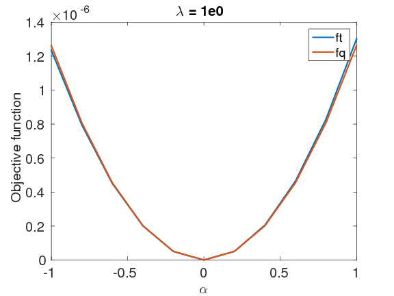
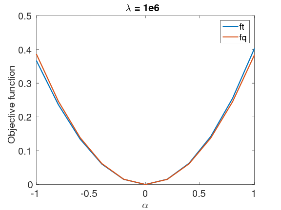
In order to test the accuracy of this approximation \(\eqref{QuadrApprx}\), we compared the behavior of the negative logarithm function of the posterior distribution \(\eqref{BayesianVARPRJ}\), \(f_t \, = \, -\log(\rhopost(\mvec))\), and that of the Gaussian distribution, \(f_q \, = \, -\log(\rho_{\text{Gauss}}(\mvec))\), around the MAP point with both small \(\lambda\), \(\lambda=1e0\) and large \(\lambda\), \(\lambda=1e6\), as shown in Figure 1. We first generate a random perturbation \(\text{d}\mvec\), with a maximum absolute value of \(0.8 \, \mathrm{km}/\mathrm{s}\). Next, we calculate the objective values \(f_t(\mvec+\alpha\text{d}\mvec)\) and \(f_q(\mvec+\alpha\text{d}\mvec)\) for \(\alpha \in [-1:0.1:1]\). In both cases, the negative logarithm function of the Gaussian approximation closely matches that of the true posterior distribution, which indicates that our approximation is accurate.

Randomize then optimize method — Given our Gaussian approximation of the posterior distribution, a standard procedure to generate samples from such a distribution is to compute the Cholesky factor of its covariance matrix, followed by applying this factor to random noise (Rue, 2001). Unfortunately, since the size of the Hessian is \(n_{\text{grid}} \times n_{\text{grid}}\), and \(n_{\text{grid}}\) is often in the range of \(10^6\) or higher, we are unable to store the Hessian explicitly, let alone compute its Cholesky factors, which is also computationally expensive.

The randomize-then-optimize (RTO) method (Solonen et al., 2014) circumvents this problem and allows us to draw samples from a given Gaussian distribution \(\rho(\mvec) \propto \exp{(-(\mvec-\mvec_{\text{MAP}})^{T}\mathbf{H}(\mvec-\mvec_{\text{MAP}}))}\), by solving the following stochastic optimization problem (Solonen et al., 2014), \[ \begin{equation} \min_{\mvec} \left\|\Lmat\mvec - (\Lmat\mvec_{\text{MAP}} + \rvec) \right\|^{2}. \label{RTOgeneral} \end{equation} \] Here, \(\Lmat\) is any full rank matrix that satisfies \(\Hmat \, = \, \Lmat^{T}\Lmat\) and \(\rvec\) is a random realization from the Gaussian distribution \(\mathcal{N}(0,\mathcal{I})\).

Fortunately, by the construction of our approximate Hessian \(\eqref{HessianWRI}\), we have the following factorization of \(\Hmat_{\text{mis}}\): \[ \begin{equation} \begin{aligned} \Hmat_{\text{mis}} &= \Lmat_{\text{mis}}^{T}\Lmat_{\text{mis}}, \\ \Lmat_{\text{mis}} &= \sigma^{-1}(\Imat + \frac{1}{\lambda^2\sigma^2}\Pmat\A^{-1}\A^{-T}\Pmat^{T})^{-\frac{1}{2}}\Pmat\A^{-1}\Gmat. \end{aligned} \label{HmisFactor} \end{equation} \] In this expression, computing the inverse square-root of \(\Imat + \frac{1}{\lambda^2\sigma^2}\Pmat\A^{-1}\A^{-T}\Pmat^{T}\) is computationally tractable because it involves a \(n_{\text{rcv}}\times n_{\text{rcv}}\) matrix, which is much smaller than the \(n_{\text{grid}} \times n_{\text{grid}}\) matrix \(\Hmat_{\text{mis}}\). With the assumption that all shots share the same receivers, we only need to compute this matrix once for each frequency. Without loss of generality, we assume that the Hessian of the prior term has a simple structure (e.g., Low rank and sparse) so that we can compute its square root \(\Lmat_{\prior}\), where \(\Hmat_{\text{prior}} = \Lmat_{\text{prior}}^{T}\Lmat_{\text{prior}}\), with a low complexity (Solonen et al., 2014). Under these assumptions, we are able to utilize the RTO method \(\eqref{RTOgeneral}\) to draw samples from the Gaussian distribution \(\mathcal{N}(\mvec_{\text{MAP}}, \Hmat^{-1})\) through replacing terms \(\Lmat\), \(\Lmat\mvec_{\text{MAP}}\) and \(\rvec\) in \(\eqref{RTOgeneral}\) by \(\begin{pmatrix} \Lmat_{\text{mis}} \\ \Lmat_{\text{prior}} \end{pmatrix}\), \(\begin{pmatrix} \Lmat_{\text{mis}}\mvec_{\text{MAP}} \\ \Lmat_{\text{prior}}\mvec_{\text{MAP}} \\ \end{pmatrix}\), and \(\begin{pmatrix} \rvec_{\mis} \\ \rvec_{\prior} \\ \end{pmatrix}\). Here, \(\rvec_{\prior}\) is a realization from Gaussian distributions \(\mathcal{N}(0,\mathcal{I}_{n_{\text{grid}} \times n_{\text{grid}}})\). \(\rvec_{\mis}\) is a realization from Gaussian distributions \(\mathcal{N}(0,\mathcal{I}_{ n_{\text{rcv}} \times n_{\text{rcv}}})\) for each shot and frequency.

Numerical experiments

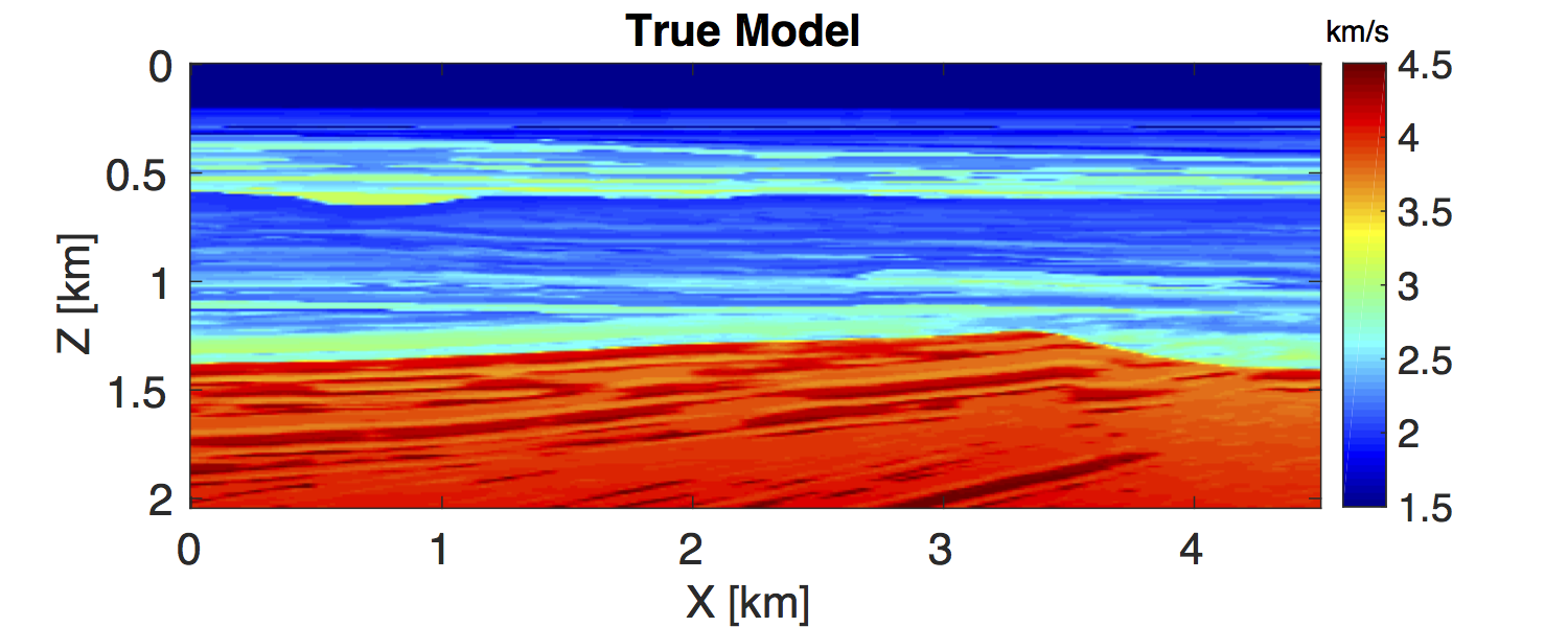
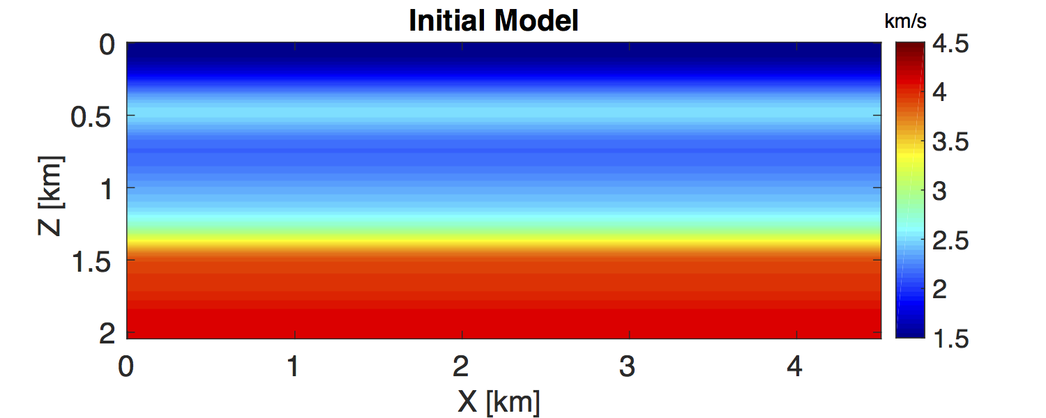
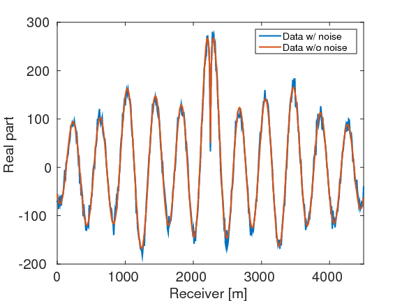
In this section, we test the feasibility of our uncertainty quantification method in a realistic seismic exploration setting. We consider the BG compass model (Li et al., 2012; Fang et al., 2015), which enjoys a large degree of variability constrained by well data. The true model and initial model are shown in the Figure 2. The model size is \(2\,\mathrm{km} \times 4.5\,\mathrm{km}\). We carry out simulations with \(91\) shot and \(451\) receiver positions sampled at \(50\, \mathrm{m}\) and \(10\, \mathrm{m}\), respectively, yielding a maximum offset of \(4.5\, \mathrm{km}\). We place all shots and receivers at the depth \(z \, = 40 \, \mathrm{m}\). According to Li et al. (2012), we carry out the inversions sequentially in 10 frequency bands ranging from \([2,\,3,\,4]\, \mathrm{Hz}\) to \([29,\,30,\,31]\, \mathrm{Hz}\) for the sake of avoiding local minima and improving convergence. The ratio of the noise and signal in the data is \(1 \, \%\) as shown in the Figure 3 and the noise level \(\sigma\) is calculated correspondingly. We select \(\lambda \, = \, 1000 \sigma\) according to the largest singular value of \(\sigma^{-1}\A^{-T}\Pmat^{T}\) with the initial model in Figure 2b (Leeuwen and Herrmann, 2015). We utilize the initial model as the prior model \(\mvec_{\prior}\), as is standard (Martin et al., 2012): \[ \begin{equation} \rhoprior(\mvec) \propto \exp (-\gamma^{-2}\|\mvec - \mvec_{\prior}\|^2). \label{PriDis} \end{equation} \] Here, we select the standard deviation \(\gamma \, = \, 2 \mathrm{km/s}\), which is larger than the maximum difference \(1.5 \, \mathrm{km/s}\) between the initial model and the true model.

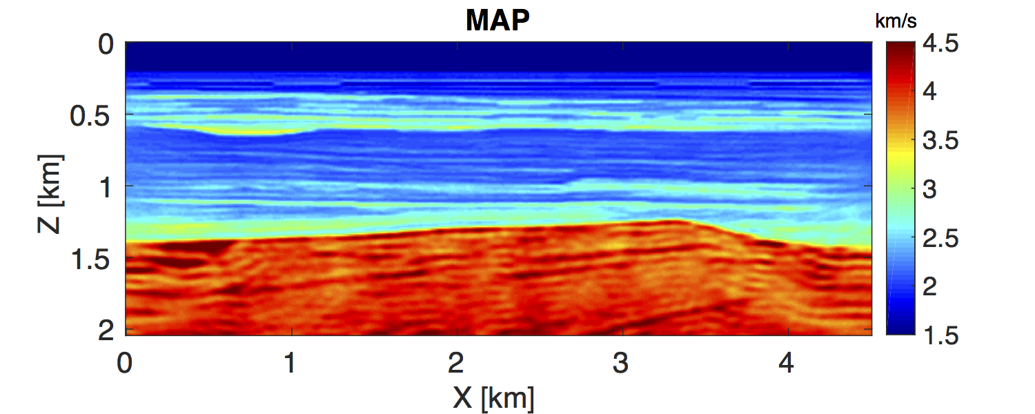
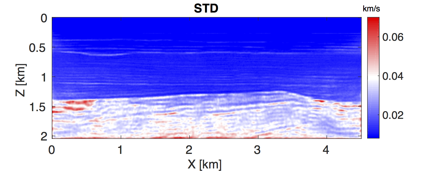
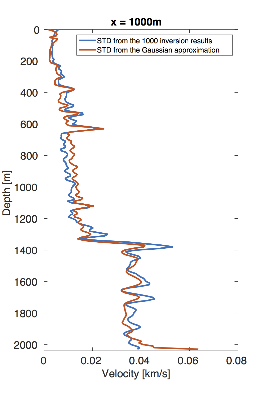
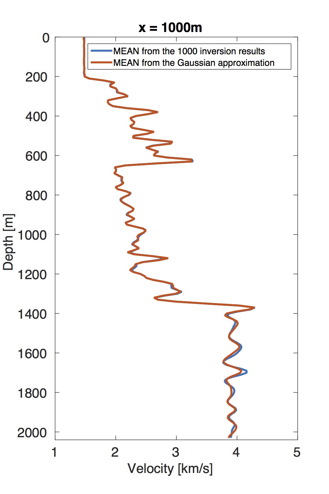
To obtain the MAP estimate, we first solve an optimization problem that corresponds to minimizing the negative logarithm function of the posterior distribution \(\eqref{BayesianVARPRJ}\), i.e., a standard WRI problem. The result is included in Figure 4a. Next, we compute the Hessian at this MAP estimate according to the Equation \(\eqref{HessianWRI}\). Finally, we draw \(1000\) samples by the RTO method \(\eqref{RTOgeneral}\) to calculate the standard deviation (STD) of the velocity model at each grid point, shown in Figure 4b. We can observe that the small level of uncertainties in the data — the \(1 \, \%\) noise — leads to the small STD, which has a maximum value of \(0.1 \, \mathrm{km/s}\). In the shallow area of the model, the STD is small, while in the deep part, it becomes large, which illustrates the uncertainties in the deep part are larger than in the shallow area. This behavior matches the fact that, compared to velocity at the deep area, the velocities in the shallow regions provide a larger contribution to the measured data. In order to validate these confidence intervals, we generate \(1000\) noisy realizations, add them to the data, and use them to generate 1000 independent inversion results, which should be samples from the true posterior distribution (Bardsley et al., 2015). We calculate the STD and mean value of these 1000 inversion results and compare to that we obtained by our approach (Figure 5) at the cross section \(x \, = \, 1000 \, \mathrm{m}\). The mean values obtained by the two approaches match each other nearly exactly. The STDs obtained by the two approaches are not as close as their corresponding mean values, but still remain reasonably stable. Considering the assumptions we made for our approach, these differences between the computed standard deviations are acceptable.

Conclusion

In this work, we proposed a semidefinite Hessian for WRI and applied it to perform uncertainty quantification. By precomputing and storing the necessary wavefields, we are able to compute the matrix-vector product of the Hessian without additional PDE solves. We used the randomize-then-optimize technique to draw samples from an Gaussian distribution that approximates the posterior distribution, and in doing so avoid forming the Hessian explicitly. As one would expect, our numerical experiment produces small uncertainties in the shallow part and large uncertainties in the deep part of the model, which matches the fact that the observed data is more sensitive to the velocity perturbation in the shallow part than in the deeper part. The STD and mean value obtained by our approach are close to those computed from the 1000 inversion results, which shows that our approach produces reasonable uncertainty analysis. Storing all these precomputed wavefields may still be a practical barrier to extending this method to the 3D case. Given the number of approximations made in the derivation of this method, further study is warranted on the approximation of the underlying density by the Gaussian density.

Acknowledgments

This work was financially supported in part by the Natural Sciences and Engineering Research Council of Canada Collaborative Research and Development Grant DNOISE II (CDRP J 375142-08). This research was carried out as part of the SINBAD II project with the support of the member organizations of the SINBAD Consortium. The authors wish to acknowledge the SENAI CIMATEC Supercomputing Center for Industrial Innovation, with support from BG Brasil and the Brazilian Authority for Oil, Gas and Biofuels (ANP), for the provision and operation of computational facilities and the commitment to invest in Research & Development.