A Unified 2D/3D Software Environment for Large Scale Time-Harmonic Full Waveform Inversion

Curt Da Silva*, Felix Herrmann
Seismic Laboratory for Imaging and Modeling (SLIM), University of British Columbia

Introduction

Given the enormous complexity associated to Full-Waveform Inversion (FWI) in terms of computational time and resources, as well as sheer code development effort, often seismic software environments are written completely in a mix of C, Fortran, and assembly language. Although these low-level languages are extremely efficient, they are also very cumbersome and can facilitate unintentional errors, and often result in codebases that are large, poorly designed and documented, and hard to maintain. From a research point of view, it can be extremely difficult for a researcher to apply and integrate their higher level algorithmic ideas to realistically sized seismic problems. Although these codes may be efficient, they are seldom tested to ensure correctness and the link between the software as-written and the mathematical underpinnings of the problem can be lost. Ultimately, hard to use and debug code can inhibit the uptake of promising research ideas into production-quality environments.

In this abstract, we propose a new organizational framework for FWI that adheres to modern software engineering principles and is flexible, efficient, and scalable. In particular, using this approach allows us to implement seemingly complicated to program mathematical algorithms such as stochastic optimization with batching in a simple and provably correct manner. The core of our software is written in Matlab, which is a programming language that allows one to write linear algebra operations in a clear and concise manner while calling efficient software packages such as BLAS and LaPACK and custom C/Fortran routines “under the hood” for solving the associated partial differential equations (PDEs). Matlab is useful precisely because it is adept at expressing high-level ideas in code and it calls other libraries that are more efficient for actual computation. This idea of separating the structural or conceptual components of the code from computational components will help us achieve the outlined goals in this software framework. We also aim to be flexible in our design, such that it is straightforward and requires little effort to integrate new components (e.g., linear solvers, preconditioners, Helmholtz discretizations, data distribution paradigms, etc.) in to the entire codebase, while simultaneously being provably correct (i.e., satisfying Taylor error estimates for the gradients , passing adjoint tests). Although we focus on frequency-domain methods, an extension of this approach to the time domain is also possible. We separate the parallelization from the serial computations, which allows us to test the serial component of our code separately and apply our code to large scale problems as easily as for small scale test problems. This decoupling also allows us to scale this approach to cloud-based computing or other heterogeneous large scale computing platforms.

Compared to the Rice Vector Library (Padula et al. (2009)), our approach is much more specific to PDE-constrained optimization problems, rather than a general multipurpose scientific computing library, and we describe more of an organizational point of view of the software rather than an implementation-specific library. The framework described in Symes et al. (2011) is similar in philosophy to our approach, but our emphasis is on flexibility. Moreover, by using Matlab, we also take advantage of using extremely efficient function handles calls, which makes code significantly more aligned with the mathematics of various algorithms, such as the multi-level Helmholtz preconditioners of Lago and Herrmann (2015), which would be very difficult to implement in C++. The Seiscope library (Métivier and Brossier (2016)) consists of a number of high-level optimization algorithms implemented in Fortran. For FWI problems, the dominant costs result from the PDE solves rather than the higher level algorithmic components themselves. Given its linear algebraic underpinnings, Matlab is well suited for expressing optimization algorithms in a compact and readable manner. As a result, it is more technically reasonable to write the higher level algorithms in Matlab and leave the lower-level components to languages such as C and Fortran.

Software organization

The standard adjoint-state method of full-waveform inversion problems involves solving \[ \begin{equation} \min_{m} \sum_{i} \dfrac{1}{2}\|P H_i(m)^{-1}q_i - D_i\|_2^2, \label{objective} \end{equation} \] where \(m\) is the model vector, \(P\) is the linear operator that restricts the wavefield to the receiver locations, \(H(m)u = q\) is the Helmholtz equation with source \(q\), and \(D\) is the observed data, where \(i\) runs over sources and all frequencies (of which there are \(n_s\) and \(n_f\), respectively).

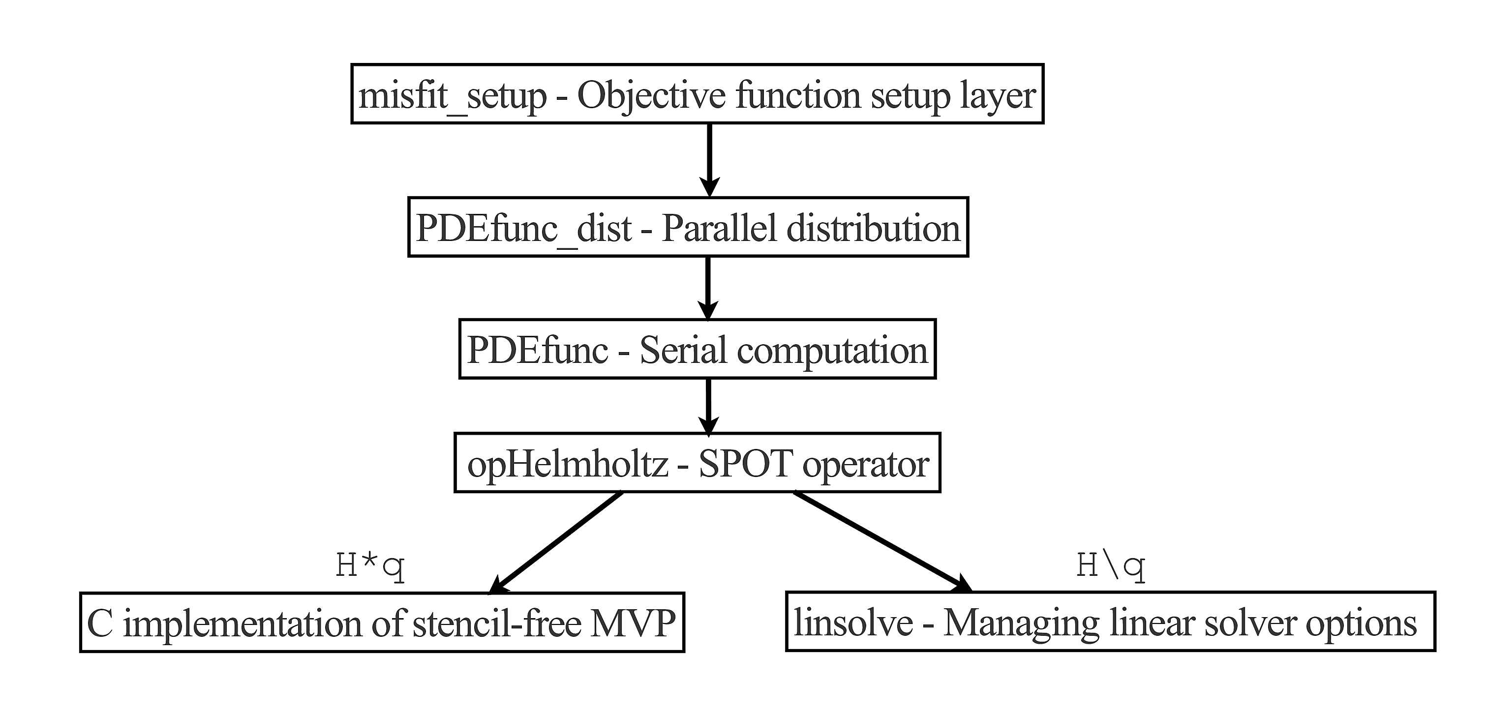
We take a hierarchical approach to the design of this environment, as shown in Figure 1. At the topmost level, our routine misfit_setup is responsible for subsampling and distributing \(D\) according to specified source and/or frequency indices, and returns a function handle to an objective function, a gradient vector, and an optional Hessian operator. This objective function handle is suitable for black-box optimization routines such as L-BFGS or Newton-based methods. This approach allows us to implement algorithms such as frequency continuation or randomized source/frequency selection in an easy manner by specifying the indices \(i\) with which we want to work at any given time. We employ the SPOT (E. van den Berg (2014)) methodology, which allows us to treat function calls as linear operators in Matlab. The Hessian operator (either full or Gauss-Newton) in this case is merely a cleverly disguised function handle, not an explicit matrix. Whenever we apply the Hessian to a vector by writing, say, \(Hess*v\), Matlab calls lower level functions to compute the Hessian-vector product and solve the corresponding PDEs, while never forming the full matrix explicitly.

The next two levels of the hierarchy consist of PDEfunc_dist and PDEfunc. PDEfunc is the general purpose serial computation function that returns various quantities depending on solutions of the Helmholtz equation, including forward modelled data, objective and gradient values, outputs of demigration and migration, as well as Gauss-Newton and full Hessian vector products. This component of the framework is responsible for “assembling” these various quantities depending on wavefields in the correct manner, as well as relying on lower level functions to actually compute these solutions. At this stage in the hierarchy, we are primarily concerned that we are arranging these component pieces properly to output the correct result, rather than dealing with the various intricacies of how to solve the Helmholtz equation iteratively. PDEfunc_dist simply computes the result of PDEfunc in an embarrassingly parallel manner, distributed over sources and frequencies, using Matlab’s distributed arrays, which are based on the Message Passing Interface (MPI) paradigm. The output is then summed across all of the workers, due to the sum-structure of the objective function in \(\eqref{objective}\).

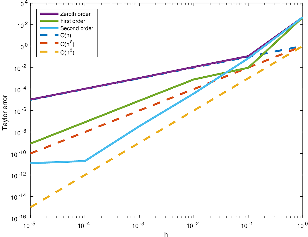
In order to validate our methods, we use the fact that, for a smooth function \(f(m)\) and an arbitrary perturbation \(\delta m\) and step size \(h\), by Taylor’s theorem, we have that the first and second order Taylor errors behave as \[ \begin{equation*} \begin{aligned} f(m_h) & - f(m) - h\nabla f(m)^T \delta m = O(h^2)\\ f(m_h) & - f(m) - h\nabla f(m)^T \delta m - \dfrac{1}{2} h^2 (\delta m)^T \nabla^2 f(m) \delta m = O(h^3), \end{aligned} \end{equation*} \] respectively, where \(m_h = m+h\delta m\). Our numerical codes do indeed reflect this theoretical behaviour for a particular range of \(h\) (modulo the effects of roundoff error and inaccuracies in the linear system solves), as shown in Figure 2. We also pass the adjoint test, which ensures that the relation \(\langle y, Ax \rangle = \langle A^Ty, x \rangle\) holds for the software implementation of a linear operator \(A\) (e.g., linearized Born-scattering, Hessian operators), and appropriately sized vectors \(x\) and \(y\), although we omit it here for brevity. Optimization algorithms exploiting smoothness properties rely on these two relationships, and lacking these properties in our codes can lead to arbitrary stalling in the optimization algorithms or can generate spurious artifacts in our results. Having our code pass these tests mitigates the possible source of issues when solving FWI problems, since our codebase is consistent with the mathematics of the problem.

Iterative inversion

Further down the hierarchy, we are concerned with the actual numerical solutions of the Helmholtz equation, which is very challenging for large wavenumbers. In particular for 3D, the large memory requirements of the model vectors and wavefields preclude us from using direct methods to solve the Helmholtz equation or even forming the matrix explicitly. The Helmholtz equation has both negative and positive eigenvalues for large wavenumbers, which makes it challenging to use off-the-shelf iterative solvers as well as in the design of preconditioners.

To discretize the Helmholtz operator, we use a stencil-based matrix-vector product written in C, with a corresponding MEX interface to Matlab, which implements the 27-pt compact stencil of Operto et al. (2007) along with its adjoint. This implementation is multi-threaded along the \(z\)-coordinate using OpenMP threads and is the only ‘low-level’ component of this software framework. The existence of these optimized routines are hidden from the rest of the Matlab code by being wrapped in the SPOT operator opHelmholtz. Again, this SPOT approach allows us to treat function calls as linear operators. When we write code like \(H*v\) in Matlab, this implicitly calls the fast C-based matrix-vector multiply, which allows us to use existing linear solvers without exposing the lower level functions underneath. This delineation of very efficient, low-level code from the higher-level components in Matlab allows us to maintain readable and easy to debug code. For 2D problems, we employ the 9pt optimal discretization of Chen et al. (2013).

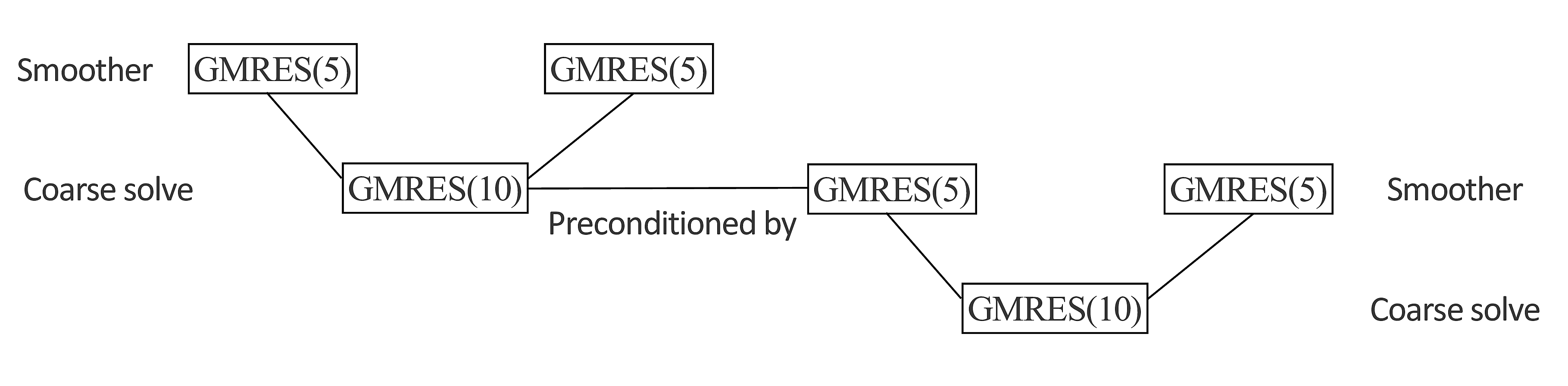
We employ a variant of the recursive multigrid preconditioner of Lago and Herrmann (2015) wherein all of the alternative smoother and coarse-grid solvers have been replaced by GMRES, displayed in Figure 3. We found that the solvers proposed by the other authors such as CGMN were not easily parallelized for stencil-free codes, despite having potentially better convergence properties, which is why we focus primarily on a preconditioning scheme that only employs highly optimized matrix-vector products.

In the hierarchy, the routine linsolve is responsible for solving \(Ax = b\) using iterative methods, given a SPOT operator \(A\), right-hand side \(b\), initial guess \(x_0\), and parameters specifying the specific method and preconditioner. This is the method called when we write \(H \backslash q\) in Matlab, as well as for various smoothing and coarse-grid solves of the multigrid preconditioner. This separation of code between matrix-vector products and matrix-vector division allows us to reuse code and make the programming of seemingly complicated preconditioners much more manageable.

We would like to emphasize that all of these implementation-specific choices are merely that, choices, and that one can easily change any and all of these decisions to suit a particular problem or computational environment. For instance, given that MPI is dependent on all nodes remaining operational for the entire duration of the computation, one can swap out the parallel Matlab component (the parallel computation) of this approach for a more fault-tolerant parallel distribution scheme, while still keeping the rest of the software design intact. The computational overhead of this approach is negligible compared to the cost of solving the forward and adjoint Helmholtz systems but we reap a significant amount of flexibility and expressibility for our algorithms in this way. Furthermore, as the state of the art advances with respect to Helmholtz discretizations and/or preconditioners, it is very straightforward to “plug in” such improvements directly in to this framework and the performance improvements will propagate throughout the entire FWI workflow. We also benefit from the integration of the 2D and 3D components of this code as we can rapidly prototype and validate FWI-based algorithms in 2D experiments, where the computational times are much more manageable, before applying them to realistic 3D problems, with very minimal code changes.

Numerical Experiments

To demonstrate the effectiveness of this software design, we validate our approach by performing stochastic optimization with batching coupled with a projected LBFGS scheme (Bertsekas (1982)). Specifically, we fix a frequency and write \[ \begin{equation} f(m,I) = \sum_{i \in I} \dfrac{1}{2}\|P H_i(m)^{-1}q_i - D_i\|_2^2, \label{frugalobj} \end{equation} \] where \(I \subset \{1, 2, \dots, n_s\}\). The stochastic optimization portion of our algorithm involves randomly subsampling the sources used, reducing the number of PDEs that need to be solved at a given iteration. Given that we have \(p\) parallel workers, the \(n_s\) sources are partitioned in to subsets \(\{S_j\}_{j=1}^p\), where the \(j^{th}\) worker has access to indices \(S_j\) of \(D\). In order to take this data distribution in to account and to minimize communication, for the \(j^{th}\) worker, at each iteration, we draw a random subset \(I_j\) of the indices it currently possesses, \(S_j\), with \(1 \le |I_j| < |S_j|\). In this way, we reduce the number of PDEs that have to be solved while still solving sufficiently many to use our parallel resources effectively (in the language of parallel computing, we are effectively “load balancing” our tasks). Once these random sources are selected, we run \(\max_{j} |S_j|/|I_j|\) iterations of an LBFGS algorithm with bound constraints on the minimum and maximum allowed velocities, as outlined in Algorithm 1. This number of iterations is chosen so that the total number of PDEs solved in the LBFGS portion of the algorithm is equivalent to one full pass through the data. This procedure then repeats with a new set of randomly drawn indices for a total of \(T\) outer iterations, which is comparable to a first-order optimization algorithm that computes \(T\) full data objective and gradient calculations, resulting in a similar runtime for both approaches. This is the so-called ‘batching’ approach in stochastic optimization, which aims to reduce the variance of a stochastic search direction by drawing a larger number of samples.

  Input: initial point \(x_0\), number of outer iterations \(T\), initial per-worker number of sources \(b_0\),

  For \(k=0,1,\dots, T\) 
  1. Each worker \(j\) draws a random set of source indicies \(I_j\) with \(|I_j| = b_k \le |S_j|\).
  2. Compute the stochastic objective \(f_k = f(x_k,I_j)\) and gradient \(g_k = g(x_k,I_j)\).
  3. Run Projected LBFGS for \(\max_{j} |S_j|/|I_j|\) iterations with minimum velocity \(\text{v}_{\min}\) and maximum velocity \(\text{v}_{\max}\)
  4. Adjust \(b_k\) if sufficient function decrease is not observed (optional)          

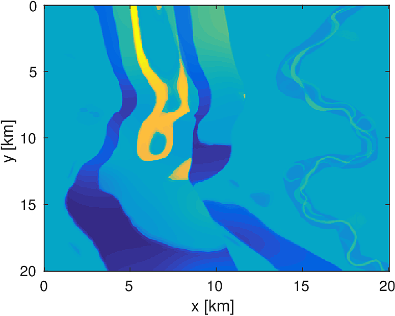
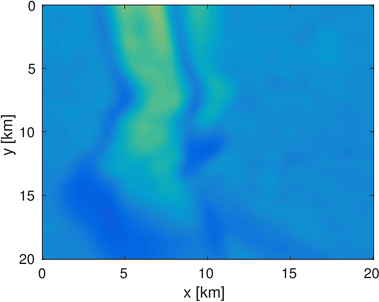
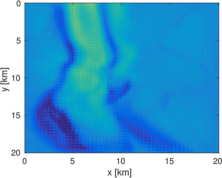
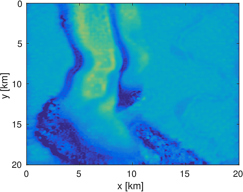
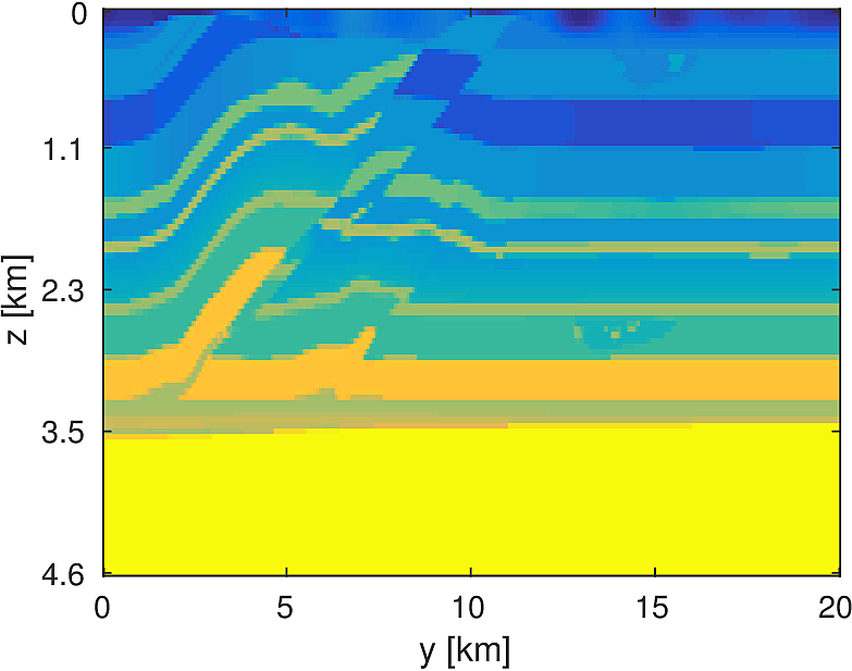
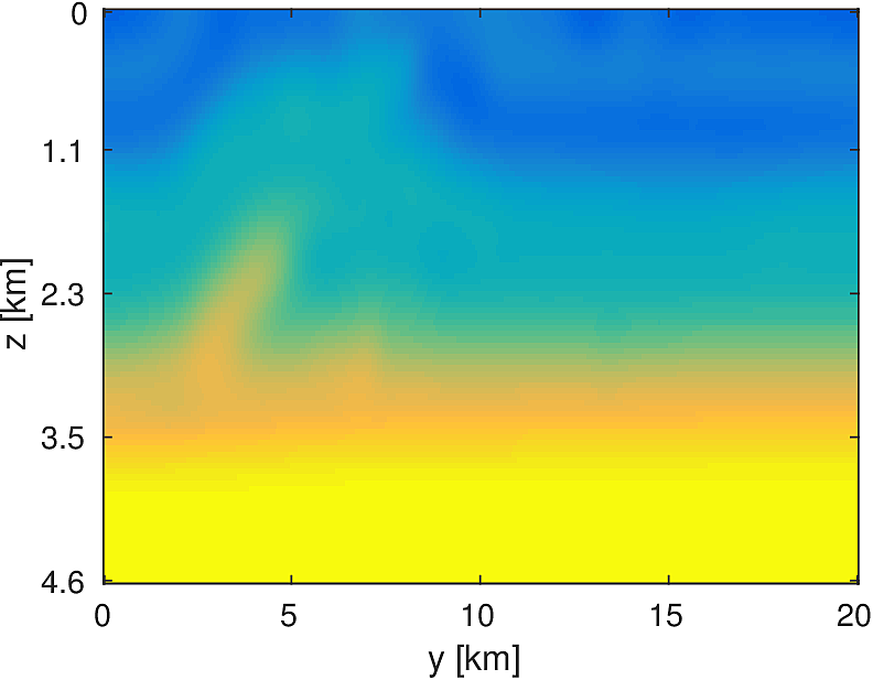
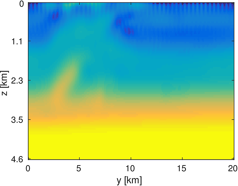
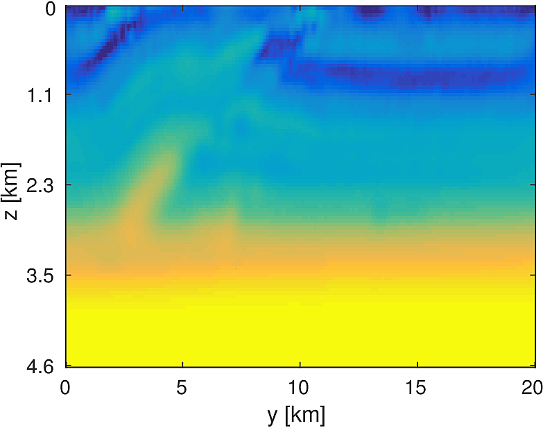
We compare this stochastic approach to a standard, full-data LBFGS method for a 20km x 20km x 4.6km subset of the overthrust model with 50m grid spacing in each dimension. We generate data from 5 frequencies from 3Hz to 7Hz and use a 50 x 50 source grid with 400m grid spacing with 400 x 400 receivers placed on a 50m spacing in an ocean bottom acquisition setup. We use 100 nodes running 4 Matlab workers each, where each node has 128GB of ram and 20 CPU cores. We invert a single frequency at a time, fixing the number of full-data objective evaluations to \(T=3\). Each worker stores 7 shots per frequency, which results in a 7-fold reduction in computational time for evaluating the stochastic objective and gradient. By allowing the stochastic algorithm to perform more iterations, we solve the same number of PDEs in both algorithms and the computational time between them is approximately the same, within a 10% margin.

Here we see that in Figures 4 and 5, given such a stringent requirement on the number of PDEs solved, the stochastic method makes much more progress towards the true solution compared to the full-data method. Also the effect of the acquisition grid imprint on the model is greatly reduced as a result of the varying set of source positions chosen at each iteration, although we have introduced some spurious noise. For a small number of passes through the data, we are able to make better progress towards the true solution using a stochastic method compared to using the full-data, although in both cases, the limited computational budget prevents the deeper parts of the model from being updated significantly. The point of these experiments is not necessarily to advocate for one algorithm over another for performing FWI, but instead to illustrate how straightforward it is to implement these algorithms for large scale FWI in this framework.

Conclusion

In this abstract, we introduced a new software framework for FWI written primarily in Matlab. We leverage Matlab’s ease of expressibility of linear algebraic concepts, as well as its ability to call highly optimized C libraries, to create a framework that is efficient, scalable, flexible, and correct. We employ modern software engineering principles to have highly organized codes that are easy to read, understand, and extend. The flexibility of our design is such that users can integrate their own existing preconditioners, Helmholtz discretizations, or data distributions in to this framework with only minor modifications. By employing these abstractions, and in particular the SPOT linear operator paradigm, we are able to easily validate research-calibre algorithms such as stochastic optimization on realistically sized problems.

This work was financially supported in part by the Natural Sciences and Engineering Research Council of Canada Collaborative Research and Development Grant DNOISE II (CDRP J 375142-08). This research was carried out as part of the SINBAD II project with the support of the member organizations of the SINBAD Consortium. The authors wish to acknowledge the SENAI CIMATEC Supercomputing Center for Industrial Innovation, with support from BG Brasil and the Brazilian Authority for Oil, Gas and Biofuels (ANP), for the provision and operation of computational facilities and the commitment to invest in Research & Development.