Time compressively sampled full-waveform inversion with stochastic optimization

Summary:

Time-domain Full-Waveform Inversion (FWI) aims to image the subsurface of the earth accurately from field recorded data and can be solved via the reduced adjoint-state method. However, this method requires access to the forward and adjoint wavefields that are meet when computing gradient updates. The challenge here is that the adjoint wavefield is computed in reverse order during time stepping and therefore requires storage or other type of mitigation because storing the full time history of the forward wavefield is too expensive in realistic 3D settings. To overcome this challenge, we propose an approximate adjoint-state method where the wavefields are subsampled randomly, which drastically the amount of storage needed. By using techniques from stochastic optimization, we control the errors induced by the subsampling. Examples of the proposed technique on a synthetic but realistic 2D model show that the subsampling-related artifacts can be reduced significantly by changing the sampling for each source after each model update. Combination of this gradient approximation with a quasi-Newton method shows virtually artifact free inversion results requiring only 5% of storage compared to saving the history at Nyquist. In addition, we avoid having to recompute the wavefields as is required by checkpointing.

Introduction

Time-domain Full-Waveform Inversion (FWI) is a well known and widely used method for acoustic inversion as its marching in time structure allows easy and memory-efficient implementation and fast solutions. The requirement to access the forward wavefield in a reverse order in time led to numerous techniques including checkpointing and optimal checkpointing strategies (Symes, 2007, Griewank and Walther (2000)), recomputing the wavefield when needed from a partial save of the time history, or boundary methods that use integrals to compute the wavefield from its full history saved at the boundary of the domain (Plessi, 2006; Clapp, 2009).

All approaches that aim to address the above problem are balancing memory requirements and computational cost of recovering the wavefield for the unknown part of the history. The method we are proposing in addition will also balance memory requirements with the accuracy of the gradient calculations. We motivate this strategy from recent insights in stochastic optimization that prove that gradients need not be accurate especially in the beginning of an iterative inversion procedure (Leeuwen and Herrmann, 2014). However, our approach differs slightly because we do not approximate the objective. Instead, we approximate the gradient by randomly subsampling the time history of the wavefield prior to correlation and applying the imaging conditions. To limit the imprint of this random subsamplings, we draw independent subsamplings for each source and after each model update. As a consequence, the subsampling-related artifacts average out as the inversion procedure progresses.

Our outline is as follows. First, we present our formulation of acoustic FWI followed by the proposed subsampling method. Next, we discuss it performance on a complex synthetic.

Acoustic full-waveform inversion (FWI)

We start by defining usual adjoint-state time-domain full-waveform inversion (FWI) for an acoustic media (Virieux and Operto, 2009). The continuous acoustic wave equation for the pressure wavefield \(u\) is define by the partial differential equation (PDE) \[ \begin{equation} m \frac{\partial^2{u}}{\partial{t}^2} - \nabla^2 u = q \label{AWE} \end{equation} \] where \(m\) is the spatial distribution of the square slowness, \(\nabla^2\) is the Laplacian and \(q\) is the source. In the following, we will only consider acoustic media only with discrete measurements, collected in the vector \(\vector{d}\), of the discrete pressure field \(\vector{u}\). Our unknown parameter is the discretized square slowness \(\vector{m}\) and we will denote by \(\vector{u}[t]=u(t \delta t)\) the discrete wavefield at discrete time \(t\) with \(n_t\) the total number of time steps.

For a single source \(\vector{q}_s\), time-domain inversion for the adjoint-state method derives from the following discrete PDE-constrained optimization problem: \[ \begin{equation} \begin{aligned} &\minim_{\vector{m},\vector{u}}\, \frac{1}{2}\norm{\vector{P}_r \vector{u} - \vector{d}} \\ &\text{subject to} \ {A}(\vector{m})\vector{u} = \vector{q}_s, \end{aligned} \label{FWI} \end{equation} \] where \(\vector{P}_r\) is the discrete projection operator restricting the synthetic wavefield to the receiver locations, \({A}(\vector{m})\) is the discretized wave equation matrix, \(\vector{u}\) is the synthetic pressure wavefield, \(\vector{q}\) is the discrete source and \(\vector{d}\) is the measured data. The parameters to be estimated are the discrete square slownessses collected in the vector \(\vector{m}=\{v_i^{-2}\}_{i=1\cdots N}\) with \(N\) the size of the discretization of the model and \(v\) the velocity. The adjoint-sate method solves the above problem by eliminating the PDE constraint and can be formulated as \[ \begin{equation} \minim_{\vector{m}} \Phi_s(\vector{m})=\frac{1}{2}\norm{\vector{P}_r {A}^{-1}(\vector{m})\vector{q}_s - \vector{d}}. \label{AS} \end{equation} \] The gradient of the above objective is given by the action of the adjoint of the Jacobian on the data residual \(\delta\vector{d} = \left(\vector{P}_r \vector{u} - \vector{d} \right)\) and reads \[ \begin{equation} \nabla\Phi_s(\vector{m})=-\sum_{t=1}^{n_t} \left\{\left((\vector{D}\vector{u}) [t] \right)^T\text{diag}(\vector{v} [t])\right\} =\vector{J}^T\delta\vector{d} \label{Gradient} \end{equation} \] where \(\vector{u}\) is the forward wavefield computed forwards in time via \[ \begin{equation} {A}(\vector{m})\vector{u} = \vector{q}_s, \label{Fw} \end{equation} \] and \(\vector{v}\) is the adjoint wavefield computed backwards in time via \[ \begin{equation} {A}^*(\vector{m}) \vector{v} = \vector{P}_r^* \delta\vector{d}. \label{Adj} \end{equation} \] In these expressions the superscript \(^T\) denotes the transpose and the matrix \(\vector{D}\) represents the discrete second-order time derivative. We define the discrete second-order time derivative as \[ \begin{equation} \frac{\partial^2 \vector{u}}{\partial t ^2} [t] = \frac{\vector{u}[t-2] -2 \vector{u}[t-1] + \vector{u}[t]}{\delta t^2} \label{der} \end{equation} \] so that the matrix \(\vector{D}\) becomes a lower-triangular matrix and its transpose an upper-triangular matrix. Given this convention, we compute the second-time derivative of the forward wavefield with the left lower-triangular derivative matrix and conversely we apply the right upper-triangular derivative matrix to the time-reversed adjoint wavefield. With this convention we match the computational order so we have the necessary wavefields at the the different times available. We put the transpose on \(D\) so we only need to store one time-step of the forward wavefield.

Assuming \(I=[1,2,3,...., n_t]\) and with the time derivative defined as in Equation \(\ref{der}\), we can write an equivalent of the gradient in Equation \(\ref{Gradient}\) as \[ \begin{equation} \nabla\Phi_s(\vector{m})=-\sum_{t \in I} \left[ \text{diag}(\vector{u}[t]) (\vector{D}^T \vector{v} [t]) \right] =\vector{J}^T\delta\vector{d}. \label{GradientAdj} \end{equation} \] The advantage of the alternative expression for the gradient, with the application of the derivative switched, is that we avoid storage of wavefield at additional time steps. While this alternative formulation is beneficial, gradient computations need storage of wavefields for all sources, which is computationally prohibitive.

Approximate FWI via stochastic gradients

The main disadvantage of time-domain adjoint state methods is the need of access to both the forward and adjoint wavefields. While certain techniques, mentioned in the introduction, overcome this need we follow a different strategy by allowing (random) errors in the gradient while still computing the objective accurately. Instead of using wavelet or other domain lossy compression techniques, we propose to randomly subsample the time histories of the forward and adjoint wavefields. In this way, we circumvent the costly recomputations part of optimal checkpointing, which requires \(\mathcal{O}(n_t\log{}n_t)\) additional computations. Before giving details on our sampling method, let us first define the subsampling rate as \[ \begin{equation} r = \frac{n_{\text{corr}}}{n_{\mathrm{Nyquist}}} \label{sub} \end{equation} \] where \(n_{\text{corr}}\) is the number of terms in the correlation calculations that are part of the gradient. Naively, these correlations are carried out over all time steps of the simulations but this not necessary since the simulation time steps are much smaller then the Nyquist sample interval. Therefore, we define our subsampling rate with respect to the \(n_{\mathrm{Nyquist}}\), which is the number of remaining terms after sampling at Nyquist.

Since we allow for errors, preferably random, in the gradient calculations we are interested in the cases where \(r\ll 1\) that require much less storage. To that end, we redefine the gradient in Equation \(\ref{GradientAdj}\) by its subsampled counterpart given by \[ \begin{equation} \tilde{\nabla}\Phi_s(\vector{m})=-\sum_{t \in \tilde{I}} \left[ \text{diag}(\vector{u}[t]) (\vector{D}^T \vector{v}[t]) \right] =\vector{\tilde{J}}^T\delta\vector{d}. \label{AGradient} \end{equation} \] In this approximation (denoted by the \(\tilde1\)), we sum over the subset of times \(\tilde{I}\subset [1\cdots n_t]\) with \(\#(\tilde{I})\ll n_{\mathrm{Nyquist}}\). To reduce the buildup of subsampling-related artifacts, we draw for each gradient step a new independent random time history for each source. As we will show below, this generated fewer artifacts compared to deterministic periodic subsampling since the artifacts from different gradient updates tend to cancel. Instead of choosing the samples uniformly random, we employ a jitter sampling technique (Hennenfent and Herrmann, 2008) to control the maximum time gaps for a given subsampling rate \(r\).

Random subsampling of the different terms in the correlation correlations is not the only way to subsample. As we have learned from the field of Compressive Sensing, we can also randomly mix and subsample the time histories. Since we do not have the complete time history available, this mixing can not be done with dense matrices but is feasible with sampling matrices \(\vector{M}\) for which \(\vector{M}^T\vector{M}\) is block diagonal. In this case, the gradient for a single shot and at a single position in the subsurface can be written as \[ \begin{equation} \tilde{\nabla}\Phi_s(\vector{m})[\vector{x}_i,\vector{y}_i,\vector{z}_i]=- \vector{u[\vector{x}_i,\vector{y}_i,\vector{z}_i]}^T \vector{M}^T \vector{M} (\vector{D}^T \vector{v[\vector{x}_i,\vector{y}_i,\vector{z}_i]}), \label{AGradienti} \end{equation} \] where \(\vector{M}\) is the time-mixing and subsampling matrix.

Line Search

In Algorithm 1, we use the weak Wolf line search in order to find the correct step length for our updates. However, remember that we are not working with the true gradient because of the subsampling. For that reason, we check whether the Wolfe line-search conditions (Skajaa, 2010) are met. We check whether the objective is decreasing and whether the curvature condition is met. If the curvature is not met but the objective is decreasing, we consider the step length to be correct. This guarantees we are still a decent direction.

Examples

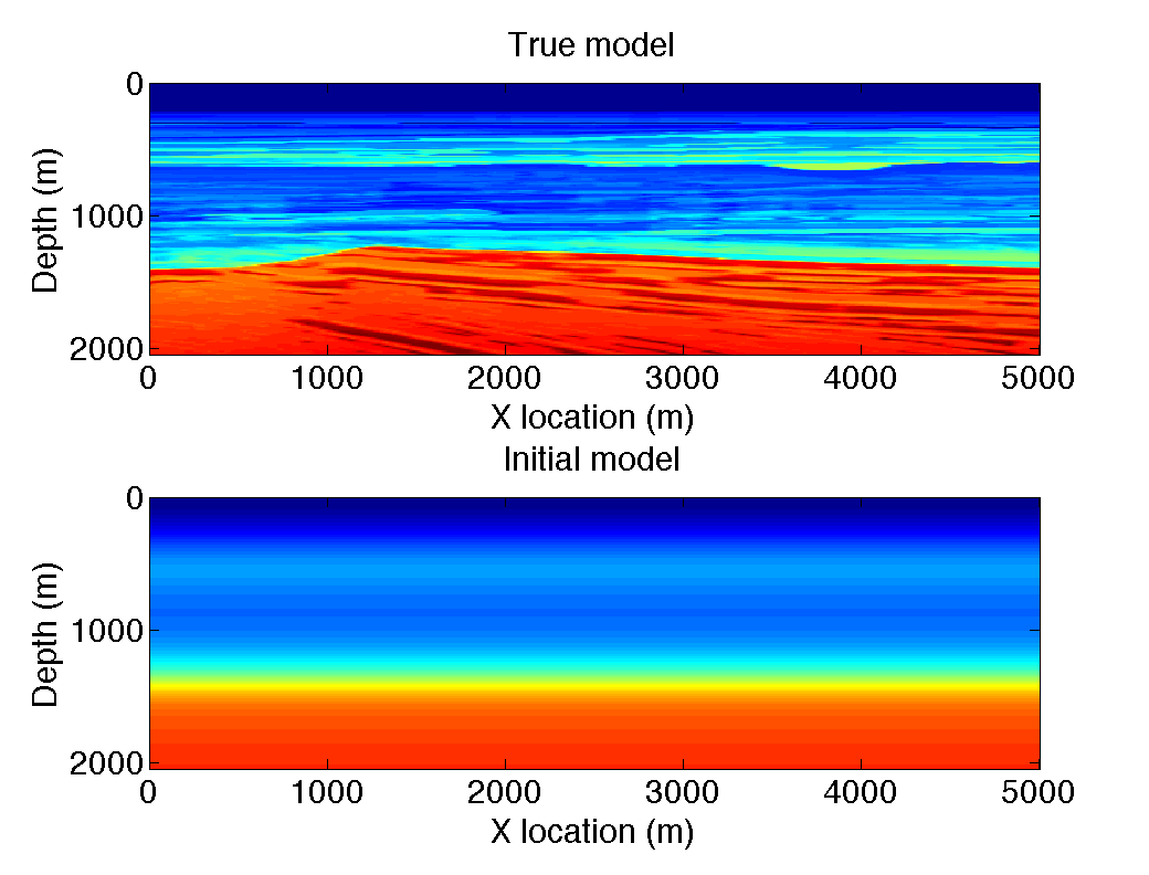
To demonstrate the performance of our stochastic optimization approach to FWI, we first consider the performance of stochastic-gradient descent. We introdruce stochasticity by random subsampling the forward and adjoint wavefield which causes random errors in the gradients but not in the objective. For a synthetic, we invert for the square slowness from pressure data recorded at the surface. We have chosen a model small enough to insure we can store the complete time history at Nyquist sampling rate. We use 50 sources at 100m intervals and 201 receivers at 25m intervals and Ricker wavelet with a 15Hz peak frequency as a source. To time step given by the CFL stability condition is \(\delta t =.5 \text{ms}\) yielding 4801 timesteps for the 2.4 s of recording. Given the central frequency of the Ricker wavelet the Nyquist sample interval is 4ms yielding \(n_{\textrm{Nyquist}}=601\). To limit the memory inprint we choose a subsampling ratio of \(r=.05\) for our approximate gradient calculations according to Algorithm 1 . This reduces the number of time samples to be stored to 30—34.

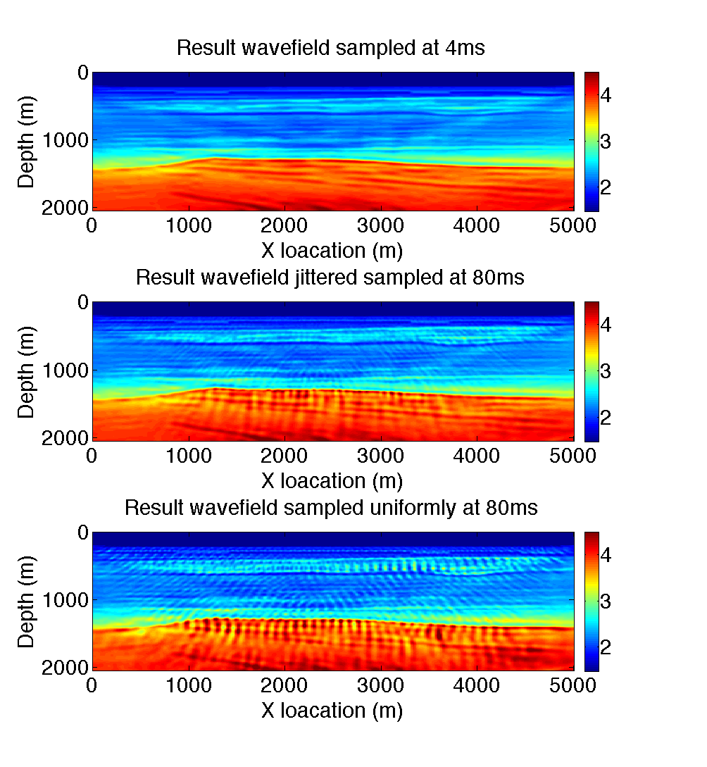
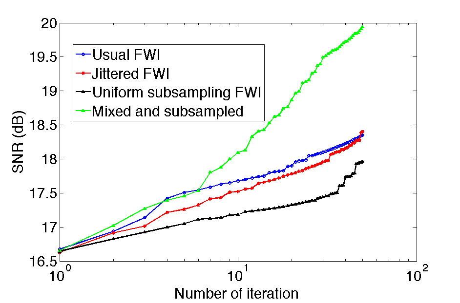
To make a fair comparison, we fixed the number of gradient steps to 50 given a a relatively good 1D starting model (see Figure {1) obtained by smoothing. We compare our subsampling methods, namely jitter sample and mixed-subsampled, to gradients calculated for correlations carried out at Nyquist. The results are summarized in Figure 2 . As we can see from this Figure, the results obtained with approximate FWI sampled at \(r=.05\) show generally the same features as the inversion result sampled at Nyquist. The artifacts appear random and relatively mundane. In Figure 3 we compare the relative model errors with respect to the true model and these plots show that periodic subsampling at \(r=0.05\) performs the worst, that Nyquist and jitter subsampled perform relatively the same throughout the iterations while the result with mixing and subsampling behaves better. This is not totally surprising because we have to remember that we mix and subsample the wavefield sampled at the time-stepping interval of the simulations, which is much smaller.

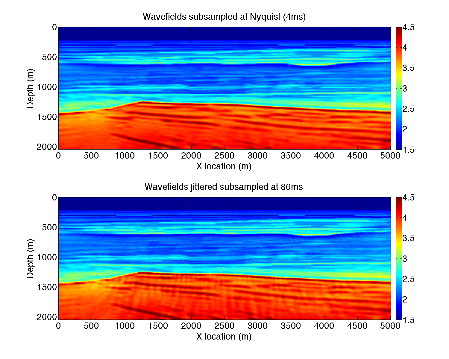
While the above example is certainly promising, it does not use second-order information. It is well-known that stochastic optimization techniques for second order method are challenging and a topic of open research. Having said that using vanilla out-of-the-box l-BFGS (Skajaa, 2010) performs remarkably well as we can observe from Figure 4, where we juxtapose results at Nyquist and at \(r=0.05\) for the jittered subsampling. It is clear from this result that the subsampling-related artifacts nearly disappeared even for the jittered sampled case. We think this remarkable because we were able to obtain this excellent result with only 5% of the time history of the forward and adjoint wavefields sampled at Nyquist. Compared the sampling rate of the simulation this is a 160-fold reduction.

Conclusions and discussion

We presented a new method to solve the time-domain adjoint-state full-waveform inversion problem without relying on complete storage or recomputation of the forward and reverse-time adjoint (receiver) wavefields. We accomplished this by combining insights from stochastic optimization and randomized subsampling where gradients are allowed to contain random sampling-related errors. Compared to random subsampling along the sources, an approach now widely used to reduces the number of wave-equation simulations, our method only approximates the gradient and not the objective by randomly subsampling the forward and adjoint wavefields prior to correlations and applying the imaging condition. We find that despite large subsampling ratios, 20-fold compared to Nyquist and 160-fold compared to the time-stepping of the simulations, excellent inversion results can be obtained by having independent samplings for each source, and possibly each gridpoint in the model, that are redrawn after each model update. The results for stochastic gradient decent clearly benefited from random sampling and we even found that the results for random mixing and subsampling were better than sampling at Nyquist. This means that the mixing picks up information at the fine time scales, which may explain the improvements in the nonlinear inversion. The results for quasi-Newton (with l-BFGS) are also excellent and show very little artifacts in case of jittered subsampling. We expect that these results will improve when we mix and subsample. As a results, we obtained an alternative method to reduce the memory and computational demands that arise from the need to have simultaneous access to the forward and reverse-time wavefield in time-domain full-waveform inversion based on time stepping.

Acknowledgements

This work was in part financially supported by the Natural Sciences and Engineering Research Council of Canada Discovery Grant (22R81254) and the Collaborative Research and Development Grant DNOISE II (375142-08). This research was carried out as part of the SINBAD II project with support from the following organizations: BG Group, BGP, CGG, Chevron, ConocoPhillips, Petrobras, PGS, WesternGeco, and Woodside.