Automatic salt delineation — Wavefield Reconstruction Inversion with convex constraints

Introduction

Time-harmonic acoustic full-waveform inversion (FWI, Tarantola (1984); Virieux and Operto (2009); F. J. Herrmann et al. (2013)) with the adjoint-state method derives from the following PDE-constrained optimization problem: \[ \begin{equation} \min_{\m,\u} \sum_{sv} \frac{1}{2}\|P \u_{sv} - \d_{sv}\|^2 \ \ \text{such that} \ \ A_v(\m)\u_{sv} = \q_{sv} \ , \label{PDEcon} \end{equation} \] where \(A_v(\m)\u_{sv} = \q_{sv}\) denotes the discretized Helmholtz equation. Let \(s = 1,...,N_s\) index the sources and \(v = 1,...,N_v\) index frequencies. We consider the model, \(\m\), which corresponds to the slowness squared, to be a real vector \(\m \in \R^{N}\), where \(N\) is the number of points in the spatial discretization. For each source and frequency, the wavefields, sources and observed data are denoted by the complex-valued vectors \(\u_{sv} \in \C^N\), \(\q_{sv} \in \C^N\) and \(\d_{sv} \in \C^{N_r}\) respectively, where \(N_r\) is the number of receivers. \(P\) is the operator that restricts the wavefields onto the receiver locations. The discretized Helmholtz matrix has the form \(A_v(\m) = \omega_v^2 \diag(\m) + L\), where \(\omega_v\) is angular frequency and \(L\) is a discrete Laplacian.

The most common approach to solve Equation \(\ref{PDEcon}\) is to eliminate the non-convex PDE constraints, which results in a parametric inversion problem over \(\m\), requiring solves of the Helmholtz and adjoint Helmholtz systems for each iteration of the optimization. While elimination of these constraints undergirds the majority of current-day FWI approaches, it is computationally expensive and prone to local minima and therefore relying on unrealistically accurate starting models. To overcome these challenges, recent work proposes to reduce computational costs via randomized subsampling techniques [(Krebs et al., 2009; Leeuwen et al., 2011; Li et al., 2012; Eldad Haber et al., 2012) and reliance on accurate starting models via so-called extensions. The goal of these extensions is to make sure that FWI does not paint itself in a corner for poor starting models that can not fit the observed data. Instead, the extended formulations are designed to fit the data irrespective of the quality (within reason) of the starting model. Symes (2008) and later Biondi and Almomin (2013) accomplish this by extending the model space to include a subsurface offset coordinate while Mike Warner’s Adaptive Waveform Inversion (AWI, Warner and Guasch, 2014) introduces Wiener filters that live in the data-space and that are designed to fit the observed data irrespective the quality of the starting model. The extended inversions, where the dimensionality of the search space is increased, are subsequently carried out by migration-velocity-analysis (MVA, Symes, 2008) type of focussing procedures that squeeze the expanded search space to something physical and thereby yielding model updates that are less prone to cycle skipping.

Wavefield Reconstruction Inversion (WRI, T. van Leeuwen and Herrmann, 2013; Leeuwen et al., 2014; Leeuwen and Herrmann, 2013) is also based on an extension. However, contrary to the afore mentioned extensions, WRI derives directly from Equation \(\ref{PDEcon}\) by replacing the constraints by \(\ell_2\)-norm penalties yielding \[ \begin{equation} \min_{\m,\u} \sum_{sv} \frac{1}{2}\|P \u_{sv} - \d_{sv}\|^2 + \frac{\lambda^2}{2}\|A_v(\m)\u_{sv} - \q_{sv}\|^2 \ . \label{penalty_formal} \end{equation} \] As opposed to conventional FWI, the optimization of Equation \(\ref{penalty_formal}\) is carried out over both the squared slownesses \(\m\) and the wavefields collected in \(\u\). As in AWI, WRI follows an alternating optimization strategy where for a fixed model \(\m^n\) at the \(n^{th}\) iteration wavefields are calculated that fit both the observed data and the PDE. Given the solution of this data-augmented wave equation given by \[ \begin{equation} \bu_{sv}= \argmin_{\u_{sv}} \frac{1}{2}\|P\u_{sv} - \d_{sv}\|^2 + \frac{\lambda^2}{2}\|A_v(\m^n)\u_{sv} - \q_{sv}\|^2, \label{ubar} \end{equation} \] the model is updated by making a step that minimizes the PDE misfit, \(\frac{1}{2}\|A_v(\m^n)\bu_{sv} - \q_{sv}\|^2\), given the solution of the data-augmented wave equation whose solutions \(\bu\) fit the observed data and the wave equation. The latter step in this alternating variable-projection approach (A. Y. Aravkin and Leeuwen, 2012), can be interpreted as a “focussing” by the wave equation itself yielding the following expressions for the gradient and Gauss-Newton Hessian (T. van Leeuwen and Herrmann, 2013): \[ \begin{equation} \g^n = \sum_{sv} \re\left\{ \lambda^2 \omega_v^2 \diag(\bu_{sv})^*\begin{pmatrix}A_v(\m^n)\bu_{sv} - \q_{sv}\end{pmatrix} \right\} \label{gradient} \end{equation} \] and \[ \begin{equation} H_{sv}^n \approx\sum_{sv} \re \left\{\lambda^2 \omega_v^4 \diag(\bu_{sv}(\m^n))^*\diag(\bu_{sv}(\m^n)\right\}. \label{Hessian} \end{equation} \] Compared to regular adjoint-state methods, the above Gauss-Newton Hessian is well approximated by the diagonal (because it is diagonally dominant) while the gradient requires only the solution of the data-augmented wave equation and is made of correlating this solution with the PDE residual. Moreover, the gradient and Hessian of WRI can be accumulated in parallel and do not require storage of all wavefields as in full-space all-at-once methods (E Haber and Ascher, 2001) used to solve Equation \(\ref{PDEcon}\). The parameter \(\lambda\) in this formulation controls the PDE and data misfits and can be chosen to fit the observed data. Given the above expressions for the gradient and Gauss-Newton Hessian, we arrive at the following expression for scaled-gradient model updates (Bertsekas, 1999): \[ \begin{equation} \begin{aligned} \dm & = \argmin_{\dm \in \R^N} \dm^T \g^n + \frac{1}{2}\dm^T H^n \dm + c_n \dm^T\dm \\ \m^{n+1} & = \m^n + \dm, \end{aligned} \label{SGD} \end{equation} \] with \(c_n\geq 0\). These updates correspond to ordinary gradient updates with \(H=0\) and and to the Newton method when \(c_n=0\) and \(H\) the true Hessian. Since the Gauss-Newton Hessian approximation (cf. Equation \(\ref{Hessian}\)) is diagonal, it can be easily incorporated into Equation \(\ref{SGD}\) at essentially no additional computational cost. For this reason, the above quadratic approximation forms the basis for our proposed generalization of WRI that includes convex constraints.

Including convex constraints

While there are strong indications that WRI is, by virtue of its increased search space and ability to fit the data, less sensitive to the accuracy of starting models, its current formulation does not employ prior knowledge in the form of convex box- or edge-promoting total-variation constraints.

Inclusion of this type of constraints makes WRI better posed and can be accomplished by simply adding convex constraints \(\m \in C\), where \(C\) is a convex set, to Equation \(\ref{SGD}\). We now have \[ \begin{equation} \begin{aligned} \dm &= \argmin_{\dm \in R^N} \dm^T \g^n + \frac{1}{2}\dm^T H^n \dm + c_n \dm^T\dm \\ &\text{ such that }\ \m^n + \dm \in C \ . \end{aligned} \label{dmcon} \end{equation} \] Incorporation of these constraints ensures that the next model iterate remains in the convex set (\(\m^{n+1} \in C\)) but makes \(\dm\) more difficult to compute. However, the problem remains tractable if \(C\) is easy to project onto or can be written as an intersection of convex constraints that are each easy to project onto. Because solving for \(\bu^n\) (Equation \(\ref{ubar}\)) is much more expensive, projections on these convex subproblems is unlikely to become a computational bottleneck. Quite the contrary, inclusion of these constraints could even speed up the overall method if it leads to fewer required model updates compared to solving the unconstrained problem.

According to Esser et al. (2013), the above approach works for fairly general Hessian approximations. For WRI specifically, where the Gauss-Newton Hessian is diagonal and made of the sum over all experiments (cf. Equation \(\ref{Hessian}\)), we only need the diagonal entries of the Hessian to be bounded for \(\m \in C\). In addition, line searches are not needed as long as \(c_n\) is small enough.

Since the approximate Hessian \(H^n\) is diagonal and positive, it is straightforward to add box constraints—i.e. the entries of the vector \(\m\) are constrained to the interval \([b, B]\) with \(b,B\) the minimum and maximum, or \(C_{\text{box}}=\{\m:\, m_i \in [b,\, B],\, i=1\cdots N\}\) for short. While inclusion of these box constraints leads to cheap closed-form analytic expressions, imposing this constraint by itself is insufficient in situations where there is lots of source cross-talk, induced by the use of simultaneous sources to speed up the computations, or in the presence of high-contrast high-velocity unconformities such as salt or basalt. As we will show below, WRI yields better solutions when adding a combination of box- and total-variation norm constraints—i.e., we seek updates \[ \begin{equation} \m^{n+1} = \m^n + \dm\quad \text{s. t.} \quad\m^{n+1}\in C_{\text{box}}\cap C_{\text{TV}}, \label{boxtv} \end{equation} \] where \(C_{\text{TV}}=\{\m:\, \|\m\|_{\text{TV}}\leq \tau\}\) with the discrete TV-norm (we reorganized \(\m\) into a \(N=N_1\times N_2\) 2D array) is defined as \[ \begin{equation} \|\m\|_{\text{TV}} = \frac{1}{h}\sum_{ij}\sqrt{(m_{i+1,j}-m_{i,j})^2 + (m_{i,j+1}-m_{i,j})^2}. \label{TVim} \end{equation} \] As we will demonstrate below, jointly imposing bound and TV constraints, the latter by constraining the TV-norm to be less than some positive parameter \(\tau\), drastically improves the performance of WRI. TV penalties are widely used in image processing to remove noise while preserving discontinuities (Rudin et al., 1992). It is also a useful regularizer in a wide variety of other inverse problems, especially when solving for piecewise constant or piecewise smooth unknowns. For example, TV regularization has been successfully used for electrical inverse tomography (E. T. Chung et al., 2005) and inverse wave propagation (Akcelik et al., 2002) and more recently in work by Guo et al. (2013). Although these approaches are somewhat similar, our formulation is different because we avoid expensive evaluations of dense Gauss-Newton Hessians. Instead, we impose the constraints in a cheap inner loop that does not involve additional wave-equation solves.

Solving the convex subproblems

A key aspect of our work is that Equation \(\ref{SGD}\), supplemented with convex constraints, is amenable to large-scale problems because it has an outer-inner loop structure. The outer loop concerns the evaluation of the expensive gradient and Hessian while the inner loop involves relatively cheap projections onto the constraints. An computationally efficient way to solve the inner convex subproblems is to modify Zhu and Chan (2008)’s primal-dual hybrid gradient method and find saddle points of the following Lagrangian (Esser et al., 2010; Chambolle and Pock, 2011; He and Yuan, 2012; Zhang et al., 2010): \[ \begin{equation} \begin{aligned} \L(\dm,\p) & = \dm^T \g + \frac{1}{2}\dm^T (H^n+2c_n\I) \dm \\ & + \p^T D(\m^n + \dm) - \tau \|\p\|_{\text{dual TV}} \end{aligned} \label{Lagrangian} \end{equation} \] for \(m^n + \dm \in C_{\text{box}}\) and \(\p\) the Lagrange multiplier. In this expression, \(\|\p\|_{\text{dual TV}}\) is the dual norm of the TV-norm, which takes the maximum instead of the sum of the \(\ell_2\)-norm of the discrete gradients (denoted by \(D\)) at each point of model \(\m\). For more details on the specific implementations of these iterations including the projections on the TV-ball of size \(\tau\), we refer to the technical report by Esser et al. (2014).

Practical aspects

The above scaled gradients with convex constraints provide the formal optimization framework with which we will carry out our experiments. Before demonstrating the performance of our approach, we discuss a number of practical considerations and strategies to expedite and terminate the iterative inversion and to make the inversion more robust to poor starting models and complex geology.

Frequency continuation. We divide the frequency spectrum into overlapping frequency bands of increasing frequency, in order to further robustify the WRI approach against cycle skipping.

Stopping criterion. As with all iterative schemes, some sort of stopping criterion is needed. For each frequency batch, we compute at most \(25\) outer iterations, each time solving the convex subproblem to convergence, stopping when \(\max(\frac{\|p^{k+1}-p^k\|}{\|p^{k+1}\|},\frac{\|\dm^{k+1}-\dm^k\|}{\|\dm^{k+1}\|}) \leq 1\e{-4}\). We compute these outer iterations as long as the reduction of the overall objective is larger than some predefined fraction of its quadratic approximation \(\dm^T \g + \frac{1}{2}\dm^T (H^n+2c_n\I) \dm \) at the current model iterate.

Acceleration by randomized sampling. To reduce the computational costs, we employ the widely-reported randomized sampling technique (Krebs et al., 2009; Leeuwen et al., 2011; Eldad Haber et al., 2012) by considering \(N_{s}' \ll N_s\) random mixtures of the sources \(q_{sv}\) defined by \[ \begin{equation} \uq_{jv} = \sum_{s=1}^{N_s} w_{js}\q_{sv} \qquad j = 1,...,N_{s}' \ , \label{simulshot} \end{equation} \] where the weights \(w_{js} \in \N(0,1)\) are drawn from a standard normal distribution. We modify the synthetic data according to \(\uds_{jv} = P A_v^{-1}(\m)\uq_{jv}\) and use the same strategy to solve the now much smaller optimization problem.

Multiple passes through the data. Despite the fact that WRI is expected to be less prone to local minima, restarting the optimizations with warm starts at the low frequencies again leads to superior results as reported by Peters et al. (2014). We employ this strategy.

Relaxation of the TV constraint. Having included constraints allows us to use a cooling technique during which the convex constraint, the TV-norm in this case, is gradually relaxed. While these type of continuation techniques have been used very successfully towards the solution of linear problems with convex constraints, devising these techniques for nonlinear problems is still a topic of open research. We found empirically that gradually relaxing the TV-constraint (\(\tau\)) during the multiple passes through the data greatly improved our results.

Numerical experiments

As we have learned from the blind Chevron Gulf of Mexico dataset, FWI is severely challenged when applied to regions with high complexity for data that miss long offsets and low frequencies (F. J. Herrmann et al., 2013). To demonstrate the added value of WRI and of adding convex constraints to FWI or WRI, we conduct a series of experiments on subsets of the 2004 BP velocity benchmark (Billette and Brandsberg-Dahl, 2005). These experiments are aimed at demonstrating the benefits of including TV-norm constraints for WRI in case of good and bad starting model, WRI compared to FWI, and multiple passes while relaxing the constraints.

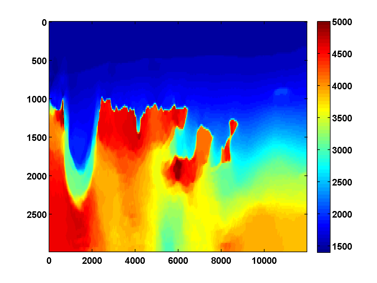
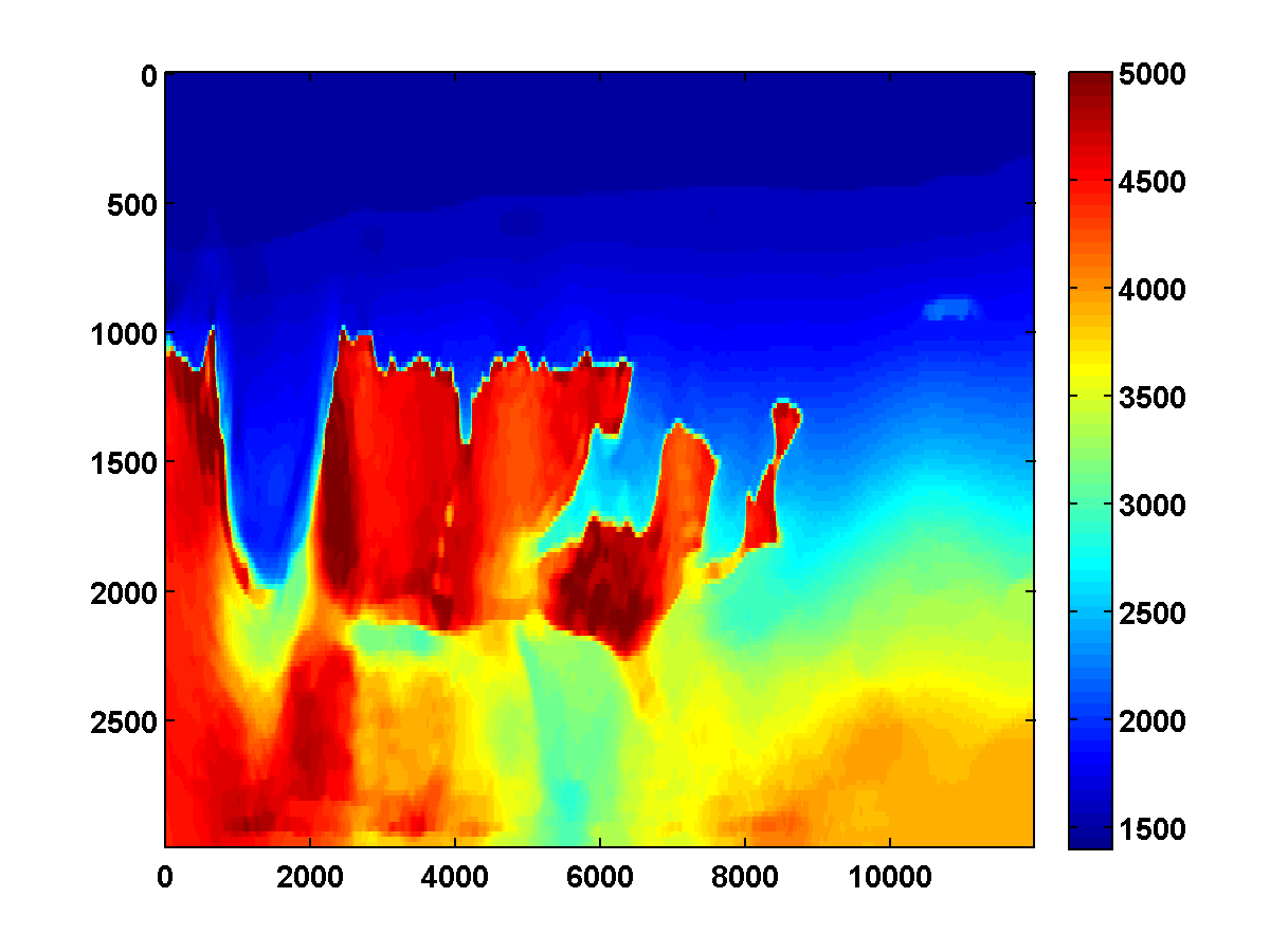
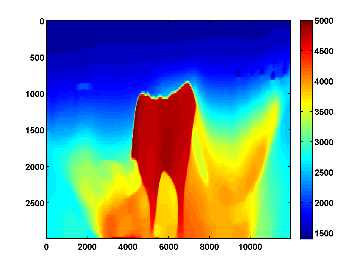
Good starting model. Let us first consider, the results of WRI with and without TV-norm regularization for the upper left part of the BP model for a starting model obtained by smoothing. The results for the first and second pass are included in Figure 1 and were obtained by carrying out the inversions from \(3\, \mathrm{Hz}\) to \(20\, \mathrm{Hz}\) in overlapping batches of two. The bound constraints on the slowness squared are defined to correspond to minimum and maximum velocities of \(1400\) and \(5000\,\mathrm{m/s}\), respectively. The \(\tau\) parameter for the TV constraint is chosen to be \(.9\) times the TV of the ground-truth model. To reduce computation time, we use only two simultaneous shots, which we redraw each time the model is updated. From these figures it is clear that including the edge-preserving TV-norm constraint greatly improves the results by removing the source crosstalk while clearly delineating the top and bottom of the salt. The figures also show that the inversion improves dramatically when making a second pass while relaxing the TV-norm constraint.

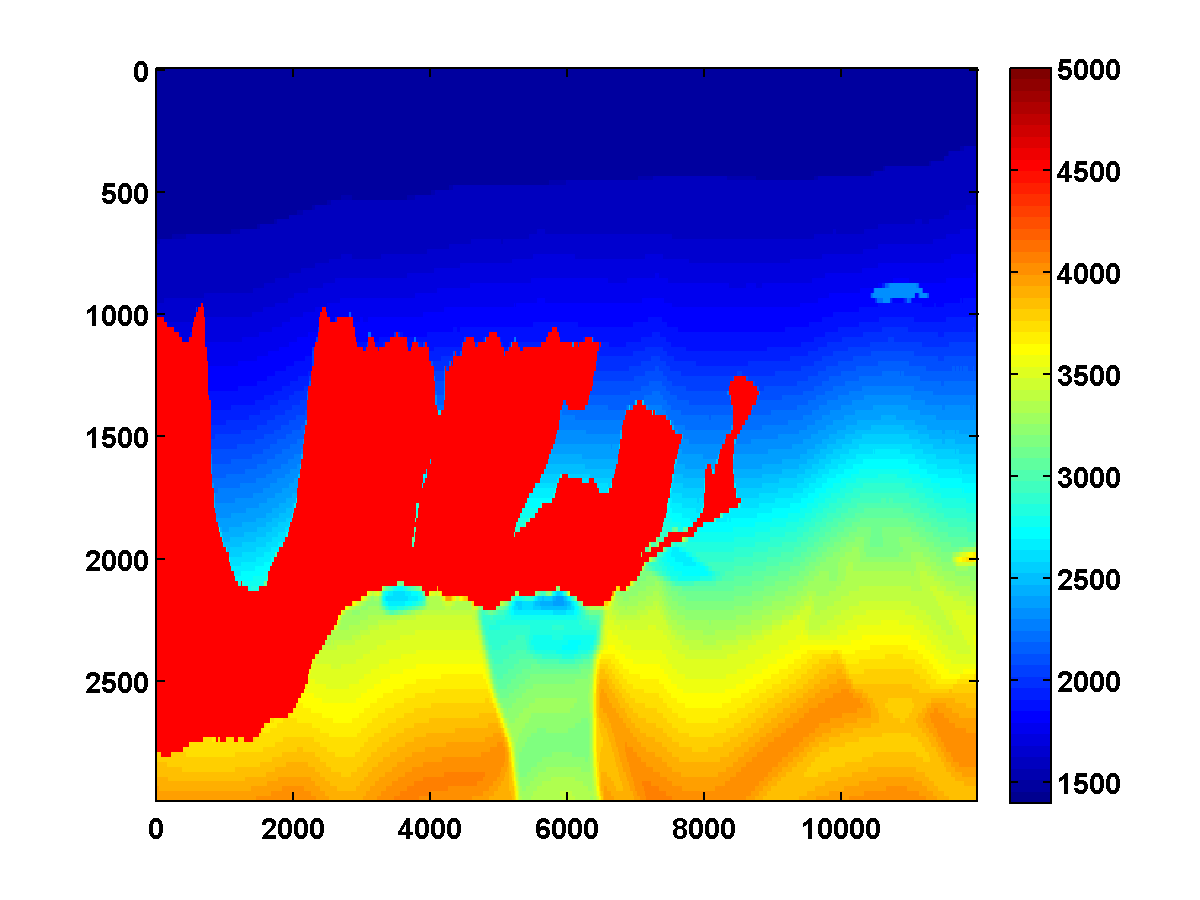
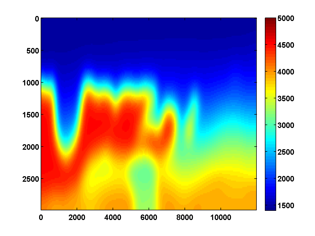
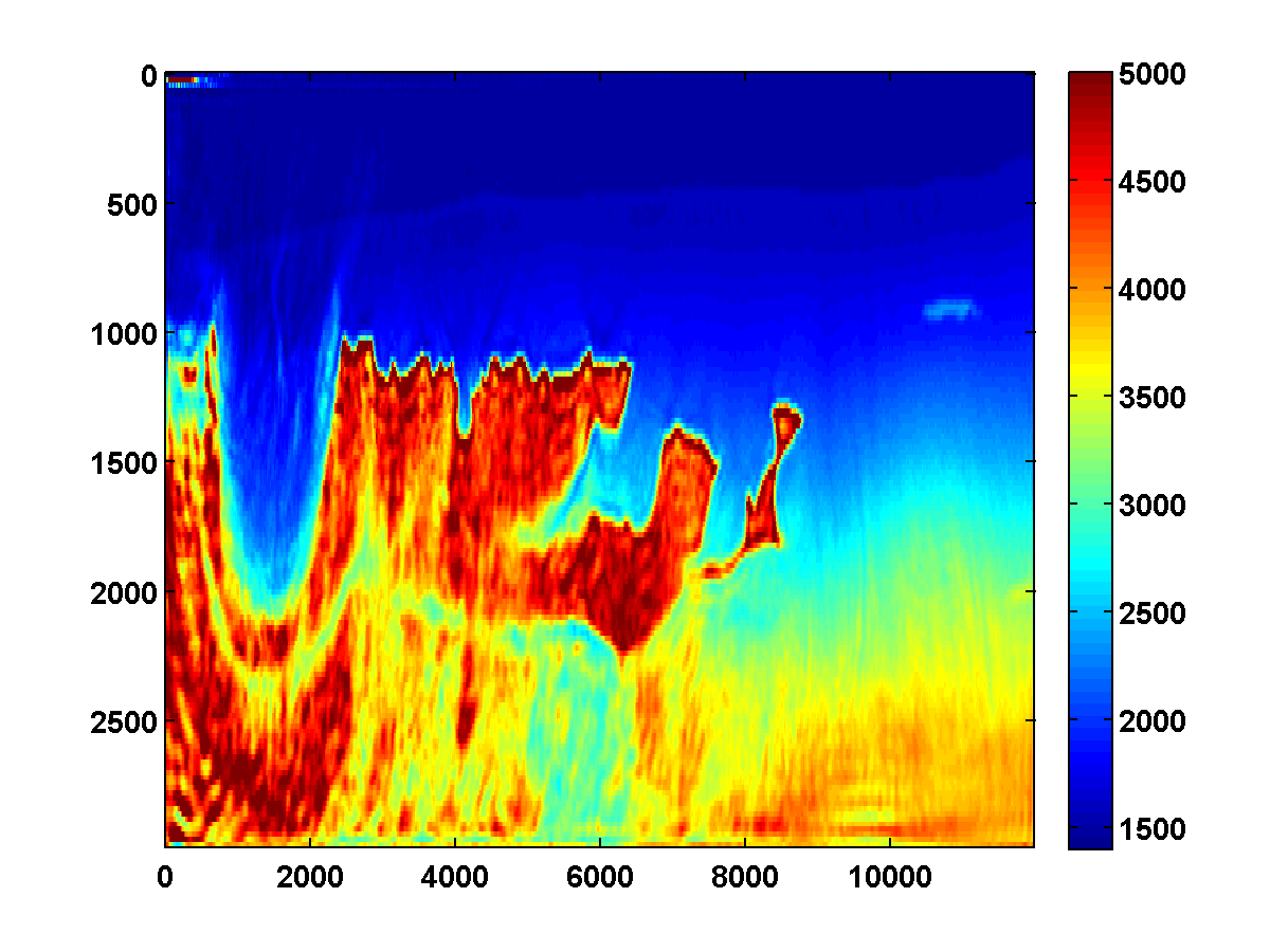
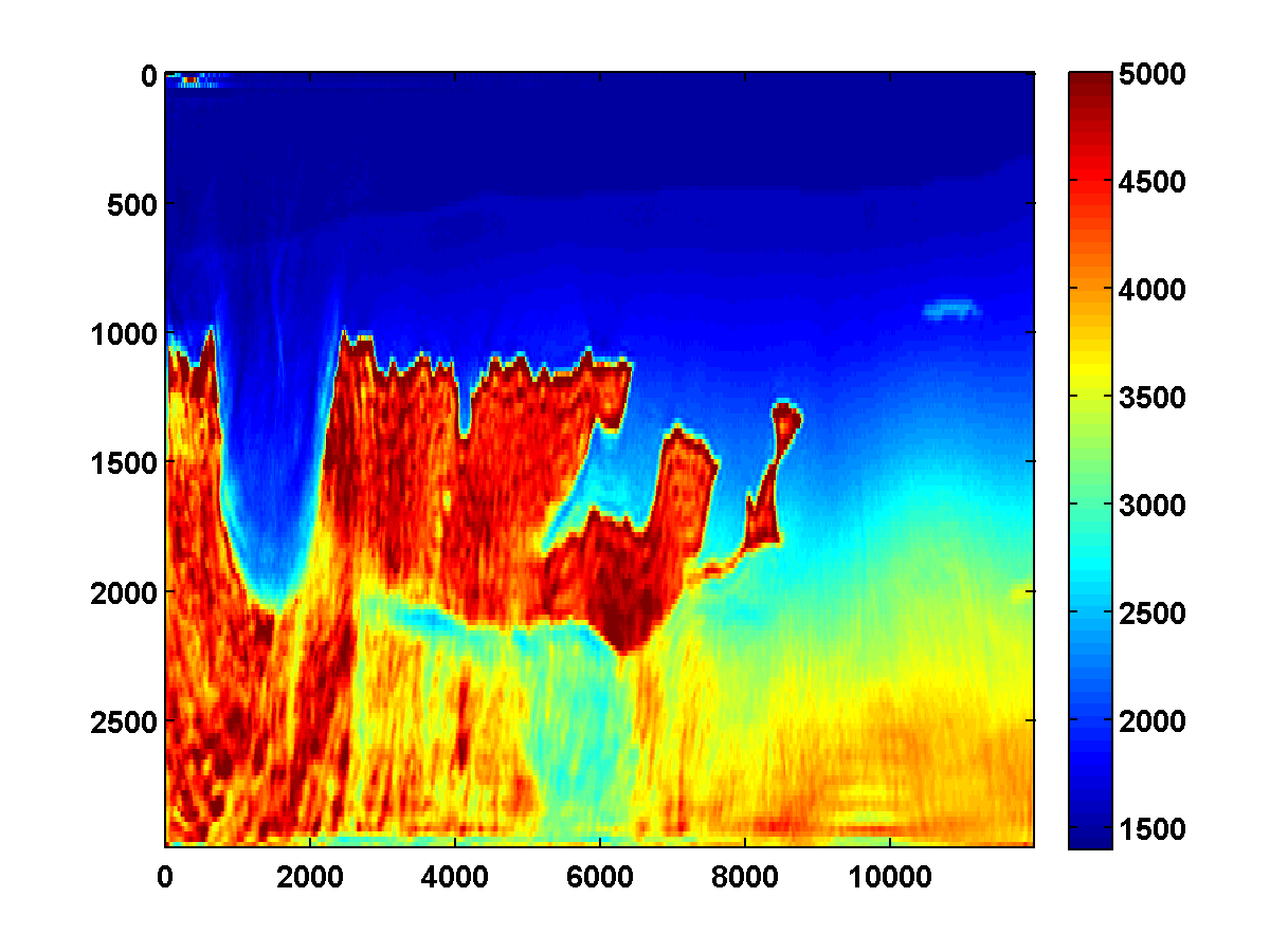
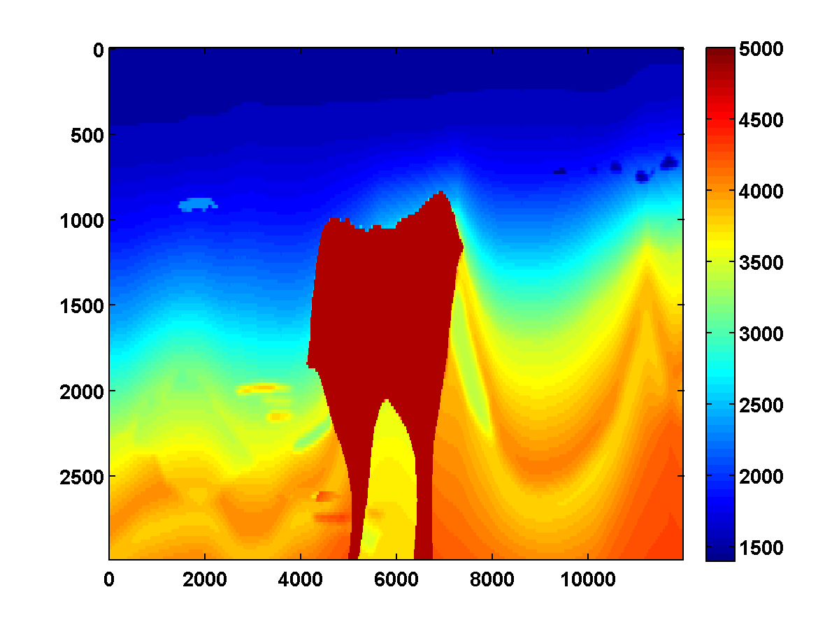
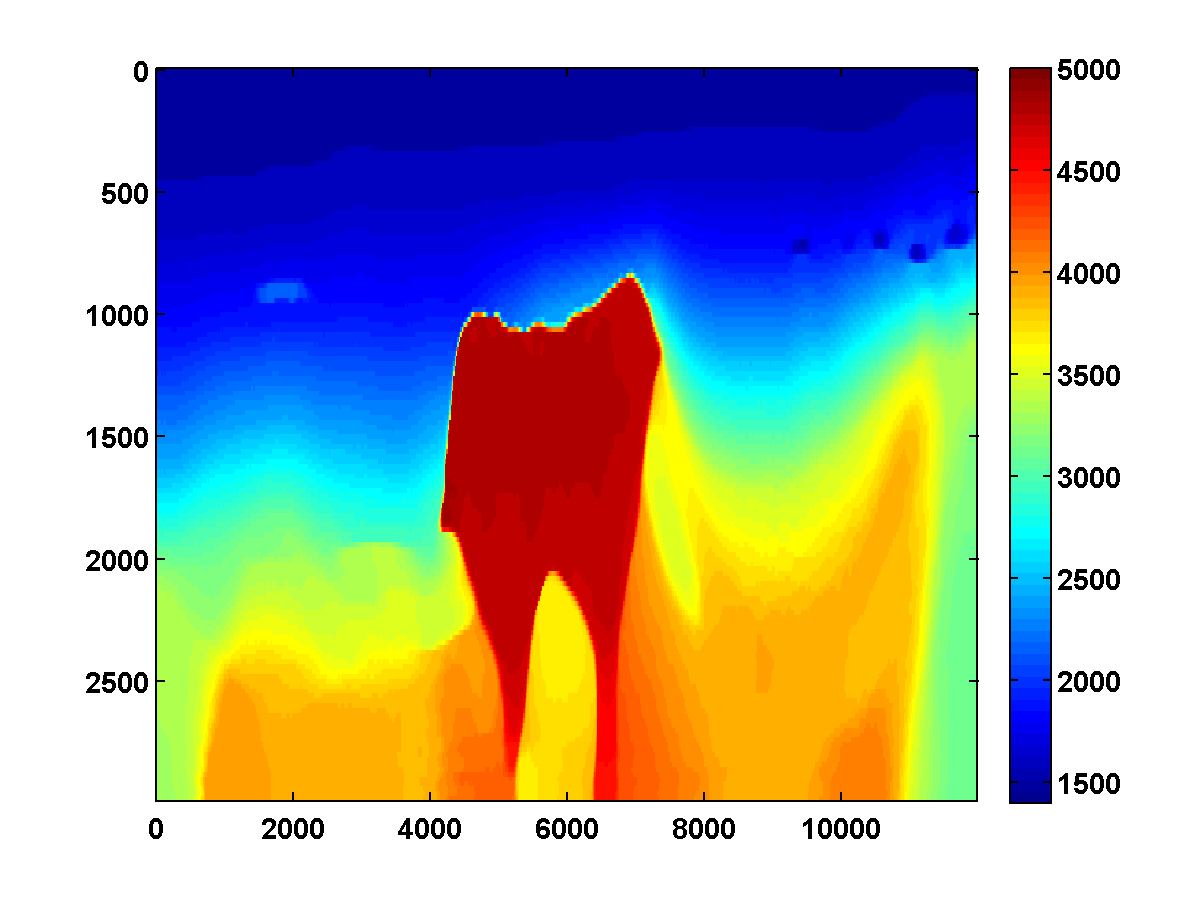
Bad initial model. As we can see from Figure 2, including TV-norm constraints also yields excellent results when starting with a model given by a simple gradient. The same applies when we approximate the Gauss-Newton Hessian of the adjoint-state method by Equation \(\ref{Hessian}\). This approximation, which is known as the pseudo Hessian, yields good but slightly inferior results compared to those of WRI. Both results were obtained via multiple passes and benefit tremendously from adding the TV-norm constraint and clearly delineate the top and bottom of the salt. (Results from adjoint-state FWI without the TV-norm constraint are very poor compared to the unconstrained WRI (not shown).)

Conclusions and future work

We presented a computationally feasible scaled-gradient projection algorithm for minimizing the quadratic penalty formulation of full-waveform inversion proposed by T. van Leeuwen and Herrmann (2013) subject to additional convex constraints. We showed in particular how to solve convex subproblems that arise when adding total-variation and bound constraints on the model. The presented synthetic experiments clearly demonstrate that full-waveform inversion in complex geological areas can greatly improve by including convex constraints. This observation applies to conventional adjoint-state FWI, Wavefield Reconstruction Inversion (WRI), and Adaptive Waveform Inversion (AWI). Both the top and bottom of the salt are well recovered, which makes the presented method a candidate to replace labour intensive salt flooding techniques. There are also indications that the TV-norm constraint improves AWI from reflection data only as reported elsewhere in these proceedings.

In future work, we still need to find a practical way of selecting the regularization parameter \(\tau\). The fact that significant discontinuities can be resolved using small \(\tau\) explains why our continuation strategy that gradually increases \(\tau\) yields improved results. These improvements stem from the fact that the TV-constraint introduces reflecting boundaries, which aid the inversion. A possible numerical framework for choosing the regularization parameter could be along the lines of the SPOR-SPG method in (Berg and Friedlander, 2011).

Acknowledgements

Ernie Esser (1980–2015), who passed away under tragic circumstances, was an extremely enthusiastic and talented researcher who was, above all, immensely generous with his time and ideas. This work is an attempt to share his work and is a reflection of what a true privilege it has been to have had the opportunity to work with Ernie. In earlier work, Ernie wished to thank Bas Peters for insights about the formulation and implementation of WRI and Polina Zheglova for helpful discussions about the boundary conditions.

This work was financially supported in part by the Natural Sciences and Engineering Research Council of Canada Collaborative Research and Development Grant DNOISE II (CDRP J 375142-08). This research was carried out as part of the SINBAD II project with support from the following organizations: BG Group, BGP, CGG, Chevron, ConocoPhillips, Petrobras, PGS, Sub Salt Solutions Ltd, WesternGeco, and Woodside.