A sparse reduced Hessian approximation for multi-parameter Wavefield Reconstruction Inversion

Introduction

Multi-parameter waveform inversion is not a new topic, (Tarantola, 1986) proposes a strategy of inverting for different parameters sequentially. Other research in multi-parameter inversion relates to multiple parameters in multiple PDE’s, such as joint inversion of electromagnetic and seismic data. In this area of research a regularization approach was used to promote structurally similar models (Gallardo & Meju, 2004). Some more recent examples in multi-parameter full waveform inversion are Lavoué, Brossier, Métivier, Garambois, & Virieux (2014) and Prieux, Brossier, Operto, & Virieux (2013).

Because regularization which promotes structural similarity relies on a priori information on the geology and sequential inversion strategies may have to be redesigned and fine-tuned for different parameters or different datasets. We will not use any of those ideas in this abstract. Although these sequential inversion and regularization concepts can definitely be very successful, we focus our efforts on fully automatic inversion with minimal use of a priori information and a minimum amount of user intervention to asses if it is a viable alternative to the methods mentioned above.

In this abstract we seek improvement on the gradient based methods (including quasi-Newton methods) by using Hessian information. Our formulation is based on the penalty formulation of the waveform inversion problem as introduced for waveform inversion by Leeuwen & Herrmann (2013). We extend their formulation to the multi-parameter case and derive a sparse Gauss-Newton type approximation to the Hessian. This type of approximation will not be possible when using the adjoint-state method to solve the Lagrangian formulation of a PDE-constrained optimization problem.

Using simple numerical experiments we illustrate the effect of our Hessian approximation and apply it to a multi-parameter waveform inversion problem.

Wavefield Reconstructing Inversion formulation

We start by defining the equations we wish to use to invert the measured waveforms. The second order partial differential equation (PDE) that describes the acoustic wave motion is \[ \begin{equation} \label{Helmholtz} \partial_r b \partial_k p + \omega^2 \kappa p = q. \end{equation} \] This is the Helmholtz equation for a lossless and isotropic medium where there are only volume-injection (monopole) sources. In this abstract we only consider measurements of the pressure field \(p\). Our unknown parameters which we want to invert are the buoyancy \(b\) and the compressibility \(\kappa\). The compressibility, buoyancy and velocity (\(c\)) in an acoustic medium are related as \(\kappa= \frac{b}{c^2}\).

The general waveform inversion problem is following PDE-constrained optimization problem (in discrete form): \[ \begin{equation} \label{prob_state} \min_{\bb,\bkappa,\bu} \frac{1}{2}\| \tensor{P} \bu- \bd\|^{2}_{2} \quad \text{s.t.} \quad \tensor{A}(\bb,\bkappa) \bu = \bq. \end{equation} \] \(\tensor{P}\) is a linear projection operator onto the receiver locations, \(\tensor{A}\) is the discretized two-paramter Helmholtz matrix, \(\bu\) is the pressure wavefield, \(\bq\) is the source term and \(\bd\) is the measured data. The two parameters to be estimated are the buoyancy \(\bb\) and the compressibility \(\bkappa\). Following Leeuwen & Herrmann (2013), we use the Wavefield Reconstructing Inversion (WRI) methodology by using the penalty objective \[ \begin{equation} \label{obj_full} \min_{\bb,\bkappa,\bu} \phi_{\lambda}(\bb,\bkappa,\bu) = \frac{1}{2}\| \tensor{P} \bu - \bd\|^{2}_{2} + \frac{\lambda^2}{2}\|\tensor{A}(\bb,\bkappa)\bu -\bq\| ^{2}_{2}. \end{equation} \] Eq.\(\ref{obj_full}\) is a combination of data-misfit and PDE-misfit, where the scalar \(\lambda\) determines the importance of each. This is now an unconstrained problem, generated by removing the PDE-constraint and adding it as a quadratic penalty term. We proceed by applying a variational projection as in Aravkin & Leeuwen (2012) to eliminate the field variable by solving \[ \begin{equation} \label{DAW} \begin{split} \bar{\bu}= \arg\min_{\bu} \bigg\| \begin{pmatrix} \lambda \tensor{A}(\bb,\bkappa) \\ \tensor{P} \end{pmatrix} \bu-\begin{pmatrix} \lambda \bq \\ \bd \end{pmatrix} \bigg\|_2 \end{split} \end{equation} \] to obtain the reduced form \[ \begin{equation} \label{objred} \min_{\bb,\bkappa} \bar{\phi}_{\lambda}(\bb,\bkappa) = \frac{1}{2}\| \tensor{P} \bar{\bu} - \bd\|^{2}_{2} + \frac{\lambda^2}{2}\|\tensor{A}(\bb,\bkappa)\bar{\bu} -\bq\| ^{2}_{2} . \end{equation} \] Using this formulation, we update the fields \(\bar{\bu}\) first, and then update the medium parameters. In other words, we first reconstruct the wavefield, given the PDE and observed data, then we use that field to update the model. So at each iteration of an optimization algorithm, we solve the least-squares problem and find an update direction using an optimization algorithm of choice. The misfit and gradients can be accumulated as a running sum over frequencies and sources. Therefore, only one field has to be in memory at a time.

To compute gradients and Hessians we need the partial derivatives of the PDE w.r.t the two parameters which are \[ \begin{equation} \label{partialderivatives} \begin{split} \tensor{G}_{\bb}={\partial \tensor{A} (\bb,\bkappa) \bar{\bu}} / {\partial \bb}\\ \tensor{G}_{\bkappa}={\partial \tensor{A} (\bb,\bkappa) \bar{\bu}} / {\partial \bkappa}. \end{split} \end{equation} \] Because of the parameterization choice, the partial derivative w.r.t one parameter does not depend on the other. These partial derivatives can be used to write down the gradient of the reduced objective function (eq.\(\ref{objred}\)): \[ \begin{equation} \label{reducedgradients} \begin{split} \nabla_{\bb} \bar{\phi}_\lambda = \lambda^2 \tensor{G}(\bb,\bar{\bu})^* \big( \tensor{A}(\bb,\bkappa)\bar{\bu} -\bq \big)\\ \nabla_{\bkappa} \bar{\phi}_\lambda = \lambda^2 \tensor{G}(\bkappa,\bar{\bu})^* \big( \tensor{A}(\bb,\bkappa)\bar{\bu} -\bq \big). \end{split} \end{equation} \] The structure of these gradients reveal that a perturbation in the compressibility will induce a nonzero gradient for the buoyancy and vice versa. This is the result of the occurrence of both parameters the Helmholtz equation and is one of the reasons multi-parameter inversion of parameters occurring in the same equation is challenging.

Obtaining a sparse approximation to the reduced Hessian without computational cost

The gradients (eq.\(\ref{reducedgradients}\)) of the reduced objective (eq.\(\ref{objred}\)) can be used for gradient descent-type methods. We will not study these, because the linear convergence rate will make this method infeasible for difficult problems with an ill-conditioned Hessian. Quasi-Newton methods can provide a faster superlinear rate of convergence. The Hessian, of which L-BFGS tries to iteratively obtain an approximation with low-rank updates, has a block structure, where the blocks corresponding to different unknowns can have widely varying Frobenius norms. This results in strong ill-conditioning (can be many orders of magnitude above machine precision). It is therefore questionable how much sense the L-BFGS approximation will make. It is possible to initialize the L-BFGS Hessian with a diagonal to correct for scale differences between Hessian blocks corresponding to the different parameters. This initialization remains a far from trivial choice that has to be made and although sensible and physically inspired choices can be made, the information is not provided by the problem at hand directly. Diagonal scaling can improve compared to the case where just the gradient is used however. See Lavoué et al. (2014) for a nice discussion about the difficulties of multi-parameter inversion and the L-BFGS Hessian. These disappointing results are the motivation to use Hessian information. We begin by deriving the Hessian matrix corresponding to the reduced objective (eq.\(\ref{objred}\)). Note that the Hessian and Newton system for the full objective (eq.\(\ref{obj_full}\)) are given by \[ \begin{equation} \label{Newton_full} \begin{aligned} \begin{pmatrix} \nabla_{\bu, \bu}^2 \phi_{\lambda} & \vline & \nabla_{\bu,\bk}^2 \phi_{\lambda} & \nabla_{\bu,\bb}^2 \phi_{\lambda}\\ \hline \nabla_{\bk, \bu}^2 \phi_{\lambda} & \vline & \nabla_{\bk,\bk}^2 \phi_{\lambda} & \nabla_{\bk,\bb}^2 \phi_{\lambda}\\ \nabla_{\bb, \bu}^2 \phi_{\lambda} & \vline & \nabla_{\bb,\bk}^2 \phi_{\lambda} & \nabla_{\bb,\bb}^2 \phi_{\lambda} \end{pmatrix} \begin{pmatrix} \delta_{\bu} \\ \delta_{\bk} \\ \delta_{\bb} \end{pmatrix} = \begin{pmatrix} \nabla_{\bu} \phi_{\lambda} \\ \nabla_{\bk} \phi_{\lambda} \\\nabla_{\bb} \phi_{\lambda} \end{pmatrix}. \end{aligned} \end{equation} \] Solving the least-squares problem in eq.\(\ref{DAW}\) is equivalent to setting the first order optimality condition of eq.\(\ref{obj_full}\) w.r.t \(\bu\) to zero: \(\nabla_{\bu}\phi_{\lambda}(\bar{\bu},\bkappa,\bb)=0\) and then applying block-Gaussian elimination for the \(\delta_{\bu}\) variable from the full Newton system (eq.\(\ref{Newton_full}\)). Another point of view is that the resulting reduced Hessian is the Schur-complement of the full Hessian. To write this compactly, partition the Hessian in eq.\(\ref{Newton_full}\) as \[ \begin{equation} \label{Hess_part} \begin{aligned} \begin{pmatrix} \tensor{E} & \tensor{B} \\ \tensor{C} & \tensor{D} \end{pmatrix}. \end{aligned} \end{equation} \] The Schur complement follows as \[ \begin{equation} \label{Schur1} \begin{split} \big( \tensor{D} - \tensor{C} \tensor{E}^{-1} \tensor{B} \big) \begin{pmatrix} \delta_{\bk} \\ \delta_{\bu} \end{pmatrix} = \begin{pmatrix} \nabla_{\bk}\phi_{\lambda} \\\nabla_{\bb}\phi_{\lambda} \end{pmatrix} - \tensor{C} \tensor{E}^{-1} \nabla_{\bu}\phi_{\lambda}(\bar{\bu},\bkappa,\bb) \end{split} \end{equation} \] which instantly simplifies to \[ \begin{equation} \label{Schur2} \begin{split} \big( \tensor{D} - \tensor{C} \tensor{E}^{-1} \tensor{B} \big) \begin{pmatrix} \delta_{\bk} \\ \delta_{\bu} \end{pmatrix} = \begin{pmatrix} \nabla_{\bk}\phi_{\lambda} \\\nabla_{\bb}\phi_{\lambda} \end{pmatrix}, \end{split} \end{equation} \] because we set \(\nabla_{\bu}\phi_{\lambda}(\bar{\bu},\bkappa,\bb)=0\) by solving eq.\(\ref{DAW}\). One of the main disadvantages of the reduced Hessians, for both penalty and Lagrangian objective formulations, is that they are dense. This can be readily observed by noting the appearance of the \(\tensor{A}^{-1}\) block in the system (see Haber, Ascher, & Oldenburg, 2000 for the reduced Hessian based on a Lagrangian objective). This results in enormous memory requirements making it usually impossible to store it in memory for medium sized 2D and larger seismic applications. The reduced dense Hessian can still be used by computing matrix-free matrix-vector products to compute the Newton direction iteratively, see Métivier, Brossier, Virieux, & Operto (2013) for this method in the waveform inversion context. Matrix-free evaluations cost expensive extra PDE or least-squares system solves. Moreover, these matrix-free matrix-vector products use a chain of linear-system solves, inducing complex and amplified error propagation. Therefore this strategy is less suitable for inexact iterative linear-system solution strategies.

The key contribution of this abstract follows here. We will make two approximations to the reduced Hessian. This Hessian originating from the penalty objective formulation can be split in a dense (\(\tensor{C} \tensor{A}^{-1} \tensor{B}\)) and a sparse part (\(\tensor{D}\)). As the first approximation, we choose to approximate the reduced Hessian by only its sparse part, \(\tensor{D}\). The accuracy of this approximation depends on the choice of the scalar \(\lambda\), it is more accurate for a small \(\lambda\). The penalty objective is equivalent to the constrained Lagrangian formulation for \(\lambda \uparrow \infty\). The use of the sparse part enables us to have it in memory and compute exact Newton-type directions at very low cost, as explained next. Thus, after the first approximation we have the following Hessian: \[ \begin{equation} \label{Hessapprox1} \begin{aligned} \begin{pmatrix} \nabla_{\bk,\bk}^2 \phi_{\lambda} & \nabla_{\bk,\bb}^2 \phi_{\lambda}\\ \nabla_{\bb,\bk}^2 \phi_{\lambda} & \nabla_{\bb,\bb}^2 \phi_{\lambda}\\ \end{pmatrix}. \end{aligned} \end{equation} \] The second approximation is to drop the off-diagonal blocks from this sparse part. These blocks can be used to obtain an algorithm which has potentially a better rate of convergence, but this topic is not explored in this abstract. Our final approximation to the reduced Hessian which we will use in the numerical examples below is given by \[ \begin{equation} \label{Hessapprox2} \begin{aligned} \tilde{\tensor{H}}= \begin{pmatrix} \nabla_{\bk,\bk}^2 \phi_{\lambda} & 0 \\ 0 & \nabla_{\bb,\bb}^2 \phi_{\lambda} \\ \end{pmatrix} = \begin{pmatrix} \tensor{G}_{\bkappa}^* \tensor{G}_{\bkappa} & 0 \\ 0 & \tensor{G}_{\bb}^* \tensor{G}_{\bb} \\ \end{pmatrix}. \end{aligned} \end{equation} \] We summarize the important properties of this Hessian approximation which we will refer to as a sparse Gauss-Newton approximation: 1) positive-definiteness, 2) Hermitian and 3) sparse. These properties make the Gauss-Newton step \[ \begin{equation} \label{GNsystem} \begin{aligned} \mathbf{p}_{gn} = \begin{pmatrix} \tensor{G}_{\bkappa}^* \tensor{G}_{\bkappa} & 0 \\ 0 & \tensor{G}_{\bb}^* \tensor{G}_{\bb} \\ \end{pmatrix}^{-1} \begin{pmatrix} \nabla_{\bb} \bar{\phi}_\lambda\\ \nabla_{\bkappa} \bar{\phi}_\lambda \end{pmatrix} \end{aligned} \end{equation} \] cheap to compute. The block structure enables parallel solution of both nonzero blocks. The content of these blocks depends of the specific parameterization and discretization used. Here we follow the disretize-then-optimize approach and discretize such that \(\tensor{G}_{\bkappa}\) is a diagonal matrix. Inverting \(\tensor{G}_{\bkappa}^* \tensor{G}_{\bkappa}\) is then trivial. The buoyancy in the Helmholtz equation (eq.\(\ref{Helmholtz}\)) is connected to differential operators and that is why the partial derivative w.r.t the buoyancy (\(\tensor{G}_{\bb}\)) will contain a differential operator. The block \(\tensor{G}_{\bb}^* \tensor{G}_{\bb}\) cannot be trivially inverted, but it is just one extra PDE-solve on top of all the linear systems that have to be solved each iteration (eq. \(\ref{DAW}\)) to obtain the fields. Note that this block is also symmetric positive definite and suitable for efficient iterative solvers and preconditioners. Therefore this sparse approximate reduced Hessian approach does not consume a lot of storage, does not take any significant computations to form and the solution of the Gauss-Newton system (eq.\(\ref{GNsystem}\)) gives rise to a minor contribution to the total computational cost of the Gauss-Newton waveform inversion algorithm. Below is the final algorithm in a nutshell.

Numerical experiments

Example 1: A motivational example

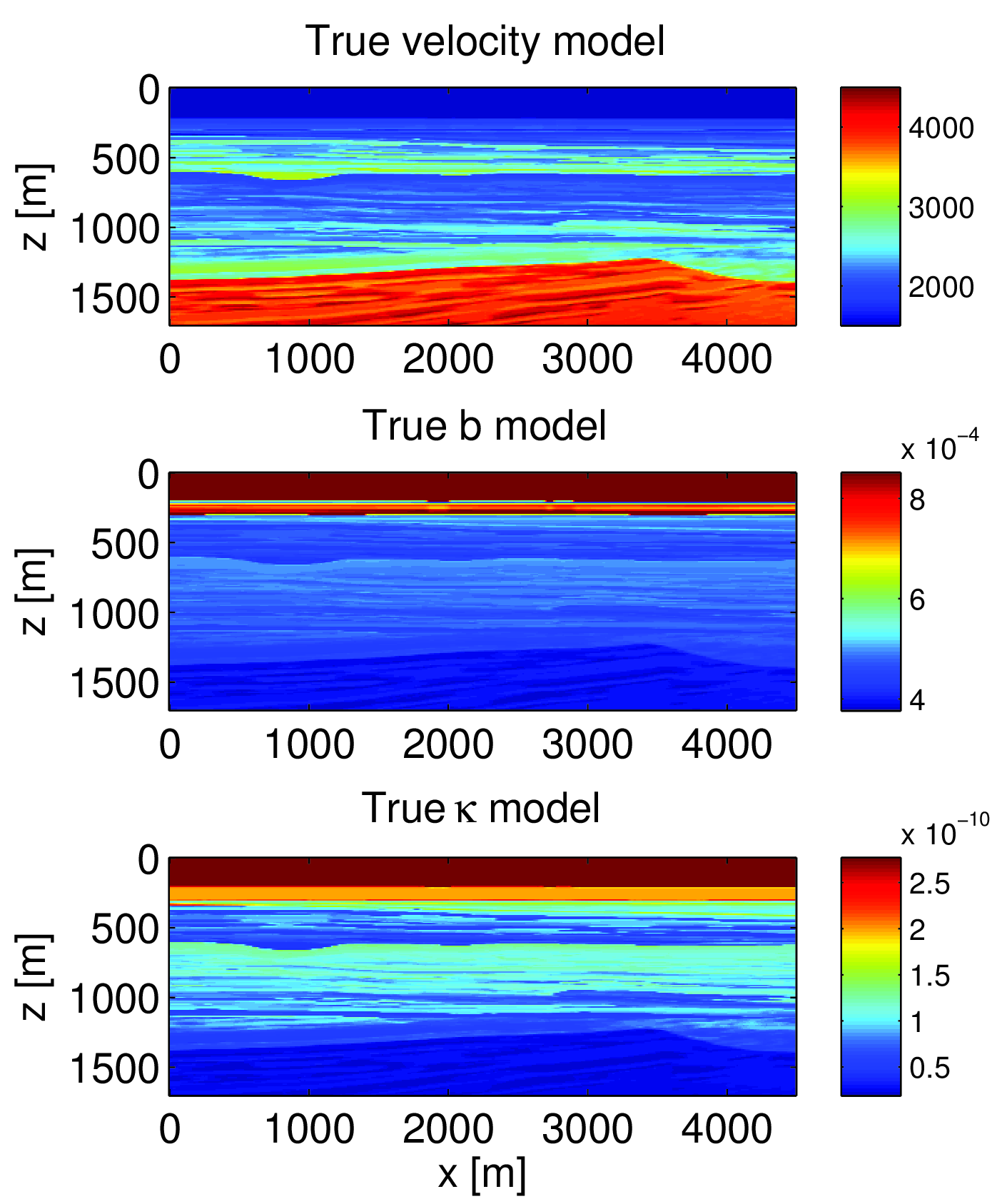
We can naively use just the gradient in the L-BFGS method. The result is shown in figure 2 where the true models are shown in figure 1. The initial guess was a smoothed version of the true models. The results show that the buoyancy is not updated very much. Nearly all of the updates is in the compressibility model. The velocity derived from the compressibility and buoyancy is actually reasonable.

Example 2: Heuristics about the effect of the sparse Hessian approximation

To analyse the effect of our proposed Hessian approximation, we construct a model with a point scatterer. It consists of both a compressibility and buoyancy perturbation. The background model is homogeneous. We look at the gradient of the objective w.r.t both the buoyancy and compressibility and compare it to the corresponding Gauss-Newton directions to visually illustrate the effect of the Hessian approximation. The sources and receivers are located at the top of the domain. We see that the Gauss-Newton direction improves the focussing of the buoyancy direction, but it does not do much for the compressibility.

Example 3: Application to waveform inversion

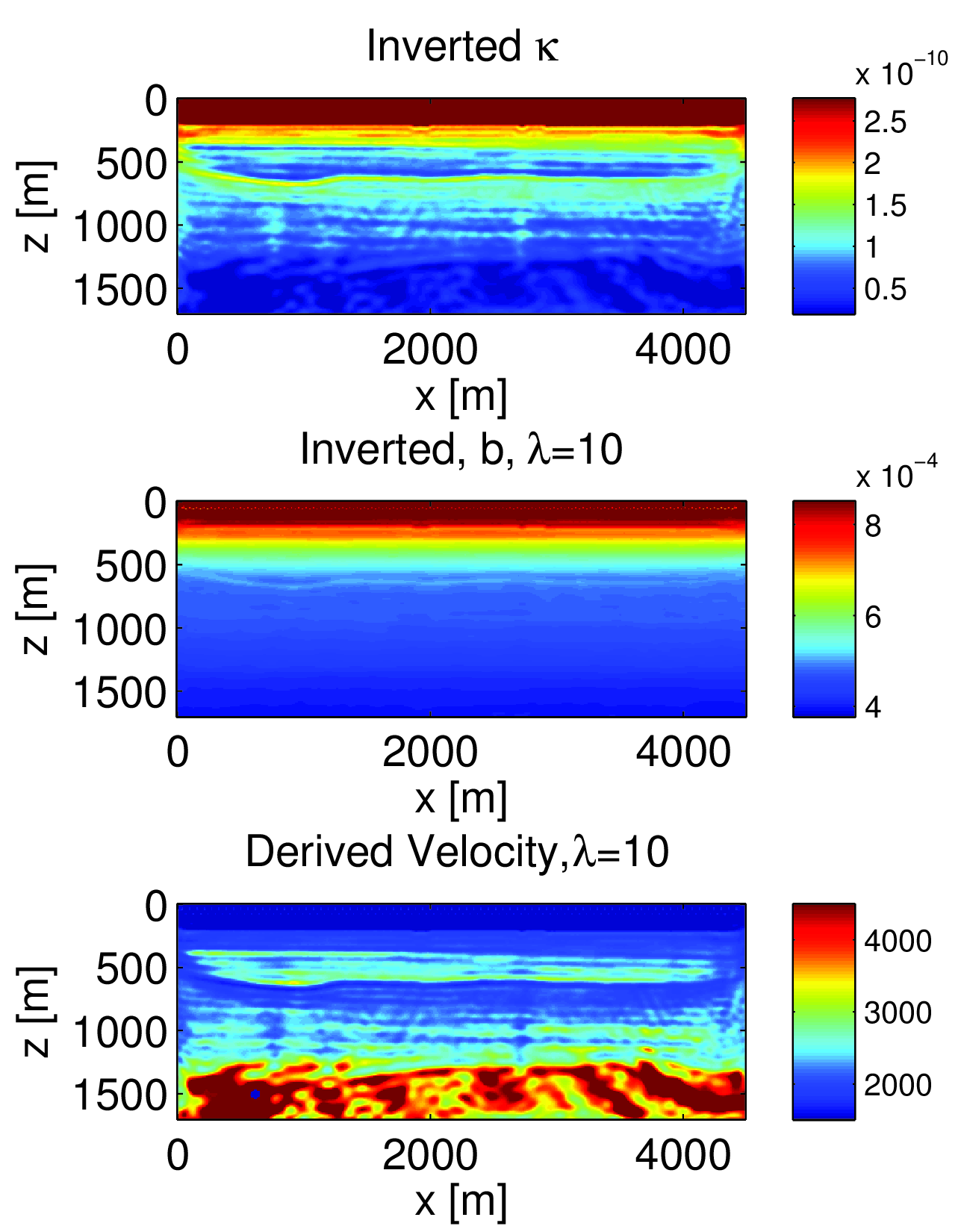
In this waveform inversion example we try to invert just pressure wavefield data recorded near the surface of the model. There are \(77\) sources and receivers and the data contains frequencies from \(2\) to \(17\) Hertz. We use a frequency continuation approach to invert the data. We invert one batch of just \(2\) frequencies at a time and use the result as an initial guess for the next batch. The batches are \(\{2, 3\}, \{3, 4\},...,\{16, 17\}\) Hertz. Algorithm 1 was used to solve this inverse problem. The results are shown in figure 4. The reconstructed buoyancy and compressibility show the main structures of the true models (figure 1). The derived velocity model is also quite decent. This synthetic example indicates that our approximate reduced Hessian allows simultaneous inversion of multiple-parameters without the introduction of explicit scalings of gradients or quasi-Newton Hessians. In a way, these type of scalings are implicit in the true Hessian which naturally provides this information based on the actual problem.

Comparison to Adjoint-State method

The adjoint-state method is based on the Lagrangian formulation to solve eq.\(\ref{prob_state}\). One proceeds by solving for the field variable and using the result to solve for the Lagrangian multiplier (adjoint-wavefield). This can be used to compute the gradient of the resulting reduced Lagrangian objective w.r.t the medium parameters. This effectively eliminated the PDE-constraint and reduced the constrained problem to an unconstrained one. The resulting reduced Hessian (see for example Haber et al., 2000) contains only one sparse part which is not Hermitian positive definite for all parameters. This makes a similar approach to the one proposed in this abstract impossible. To use Hessian information in this case, the dense Hessian needs to be stored or matrix-vector products have to be computed though, accurate and expensive, extra PDE-solves.

Conclusions and discussion

We derived a sparse approximation to the reduced Hessian based on a penalty formulation of the waveform inversion problem. This approximate Hessian enables multi-parameter waveform inversion without the need for incorporating a priori information about the coupling between the parameters by regularization, scaling of gradients or quasi-Newton Hessians or inverting for different parameters sequentially. The derived approximation to the reduced Hessian is Hermitian positive definite by construction and easy to invert when computing the update direction. Further research will focus on including more sparse parts into the approximation as well as the analysis of the practically achievable rate of convergence.

Acknowledgements

This work was financially supported in part by the Natural Sciences and Engineering Research Council of Canada Discovery Grant (RGPIN 261641-06) and the Collaborative Research and Development Grant DNOISE II (CDRP J 375142-08). This research was carried out as part of the SINBAD II project with support from the following organizations: BG Group, BGP, BP, Chevron, ConocoPhillips, CGG, ION GXT, Petrobras, PGS, Statoil, Total SA, WesternGeco, Woodside.

References

Aravkin, A. Y., & Leeuwen, T. van. (2012). Estimating nuisance parameters in inverse problems. Inverse Problems, 28(11), 115016.
Gallardo, L. A., & Meju, M. A. (2004). Joint two-dimensional dC resistivity and seismic travel time inversion with cross-gradients constraints. Journal of Geophysical Research: Solid Earth, 109(B3), n/a–n/a. doi:10.1029/2003JB002716
Haber, E., Ascher, U. M., & Oldenburg, D. (2000). On optimization techniques for solving nonlinear inverse problems. Inverse Problems, 16(5), 1263–1280. doi:10.1088/0266-5611/16/5/309
Lavoué, F., Brossier, R., Métivier, L., Garambois, S., & Virieux, J. (2014). Two-dimensional permittivity and conductivity imaging by full waveform inversion of multioffset gPR data: a frequency-domain quasi-newton approach. Geophysical Journal International, 197(1), 248–268. doi:10.1093/gji/ggt528
Leeuwen, T. van, & Herrmann, F. J. (2013). Mitigating local minima in full-waveform inversion by expanding the search space. Geophysical Journal International, 195, 661–667. doi:10.1093/gji/ggt258
Métivier, L., Brossier, R., Virieux, J., & Operto, S. (2013). Full waveform inversion and the truncated newton method. SIAM Journal on Scientific Computing, 35(2), B401–B437. doi:10.1137/120877854
Prieux, V., Brossier, R., Operto, S., & Virieux, J. (2013). Multiparameter full waveform inversion of multicomponent ocean-bottom-cable data from the valhall field. part 1: imaging compressional wave speed, density and attenuation. Geophysical Journal International, 194(3), 1640–1664. doi:10.1093/gji/ggt177
Tarantola, A. (1986). A strategy for nonlinear elastic inversion of seismic reflection data. GEOPHYSICS, 51(10), 1893–1903. doi:10.1190/1.1442046