Randomized sampling without repetition in time-lapse seismic surveys

F. Oghenekohwo^*, R. Kumar, and F. J. Herrmann
Seismic Laboratory for Imaging and Modeling (SLIM), University of British Columbia, Canada

Introduction

Repeatability in acquisition and processing ranks highest among the technical challenges faced with time-lapse seismic studies (Lumley & Behrens, 1998) and researchers continue to develop methods that will address these challenges. Computing weak 4-D signals pose another significant challenge the industry currently faces as the signal is below the non-repeatable noise introduced during acquistion or processing. Therefore, many studies have been focused on improving repeatability levels of acquired and processed time-lapse data (Eiken, Haugen, Schonewille, & Duijndam, 2003; Landrø, 1999; Porter-Hirsche & Hirsche, 1998). Recently, permanent monitoring systems have been used to acquire multiple time-lapse data and automated systems are being designed to improve the accuracy and repeatability of time-lapse surveys (Brown & Paulsen, 2011; Eggenberger, Christie, Manen, & Vassallo, 2014). Although these systems improve the repeatability levels of the time-lapse data, they are very expensive to maintain and enormous effort is required for their operation. In our recent study (Oghenekohwo, Esser, & Herrmann, 2014), we show how the concern for repeatability can be relaxed provided we randomly sample the shots during the time-lapse surveys. Consequently, we solve an inverse problem, exploiting the shared information in the baseline and monitor data, to recover a densely sampled time-lapse data from the measured randomized data. The net result was a high-fidelity 4D signal in the data domain.

Few studies involving a joint processing or inversion scheme for imaging time-lapse data have been conducted. Rickett & Lumley (2001) proposed a cross-equalization data processing flow where data repeatability is matched at each processing step, while Ayeni, Tang, Biondi, & others (2009) imaged time-lapse data acquired from simultaneous source (or blended acquisition) which is a variant of randomized marine acquisition. However, while the cross-equalization approach does not address data which has been randomly sampled without repetition, and the inversion scheme does not account for the shared information in the data sets, we exploit both requirements in our formulation to improve the 4D signal recovery quality.

In this paper, we extend our independent and joint recovery methods to the computation of time-lapse images using our randomized sampling scheme without repetition, having observed its’ efficacy to recover reliable 4D signals in the data domain. For simplicity, we show the computation of time-lapse stacked sections including 4D difference stacked sections, from randomized, subsampled baseline and monitor data.

Methodology

Given an earth model \(\textbf{m}\), the conventional approach to modeling seismic data \(\textbf{y}\) from a modeling operator \(\textbf{F}\) is: \[ \begin{equation} \label{mod} \textbf{Fm} = \textbf{y}. \end{equation} \] Ideally, \(\textbf{F}\) is either an elastic or acoustic wave-equation operator, however, for simplicity (but without generality), we redefine \(\textbf{F} = \textbf{M}^{\textbf{H}}\textbf{N}^{\textbf{H}}\textbf{S}^{\textbf{H}}\) as a linear operator mapping a stacked time section to a pre-stack seismic data volume. Here, \(\textbf{M}\) is the midpoint-offset to source-receiver operator, and \(\textbf{S}\) is the stacking operator. This linear mapping relies on the prior knowledge of the stacking velocities. This is required for constructing the normal move-out (NMO) operator \(\textbf{N}\). This velocity requirement is true with any imaging or stacking algorithm. Incorrect background velocity model or stacking velocities can lead to significant misalignments of reflectors in a migrated image or stacked section respectively, therefore it is important to have an accurate estimate of the velocity. The earth model can also be represented as \(\textbf{m} = \textbf{C}^{\textbf{H}}\textbf{x}\), where \(\textbf{x}\) is the sparse representation of \(\textbf{m}\), and \(\textbf{C}^{\textbf{H}}\) is the synthesis curvelet operator linking the model to the curvelet coefficients. Taking \(\textbf{m}\) to be the stacked time section, and combining the curvelet representation of the model with the redefined modeling operator \(\textbf{F}\), equation \(\eqref{mod}\) can be recast as : \[ \begin{equation} \label{mod2} \textbf{Ax} = \textbf{F}\text{C}^{\textbf{H}}\textbf{x} = \textbf{y}. \end{equation} \] Clearly, this formulation gives rise to an over-determined system of equations, where the observed data \(\textbf{y}\) has a higher dimension compared to the model \(\textbf{m}\). An inversion approach is typically required to find an estimate \(\tilde{\textbf{m}}\) of the true model \(\textbf{m}\), given the observed data. Inversion for the stacked section of a seismic data is a viable approach as it affords us to sample as little as possible since the number of unknowns in our linear system of equations is small. Furthermore, we note that the estimation of the stacked sections from the observed data is significantly less computationally expensive than recovering the complete wavefield. The inversion can be done in several ways and in consistency with our previous work, we will adopt the \(\ell_1\) inversion procedure where we promote sparsity in \(\textbf{x}\) by solving the convex optimization problem: \[ \begin{equation*} \tilde{\textbf{x}} = \arg \min_{\textbf{x}}\|\textbf{x}\|_1 \quad \text{subject to} \quad \textbf{y} = \textbf{A}\textbf{x}. \nonumber \end{equation*} \] For time-lapse studies, where we have at least a baseline pre-stack data \(\textbf{y}_1\) and a monitor pre-stack data \(\textbf{y}_2\), we can do two things : (1) inversion of the data sets to obtain an estimate of the stacked section for the baseline \(\tilde{\textbf{m}}_1= \textbf{C}^{\textbf{H}}\tilde{\textbf{x}}_1\) , the monitor \(\tilde{\textbf{m}}_2= \textbf{C}^{\textbf{H}}\tilde{\textbf{x}}_2\) , and finally differencing the two stacked sections. (2) inversion of the difference between the pre-stack baseline and monitor data (provided the data are matched to a common computational grid), to obtain the time-lapse stacked section. The problem formulation allows us to employ our independent recovery strategy (IRS) and joint recovery method (JRM), discussed in (Oghenekohwo et al., 2014), to estimate the individual stacked sections and the corresponding 4D stacked sections. The IRS simply inverts for the baseline and monitor stacked sections independently, by solving the following problems \[ \begin{equation*} \begin{aligned} \nonumber \tilde{\textbf{x}}_1 & = & \arg \min_{\textbf{x}_2}\|\textbf{x}_1\|_1 \quad \text{subject to} \quad \textbf{y}_1 = \textbf{A}_1\textbf{x}_1\\ \nonumber \tilde{\textbf{x}}_2 & = & \arg \min_{\textbf{x}_2}\|\textbf{x}_2\|_1 \quad \text{subject to} \quad \textbf{y}_2 = \textbf{A}_2\textbf{x}_2 \end{aligned} \end{equation*} \] On the other hand, the JRM performs a joint inversion by taking into account the shared information (Baron, Duarte, Sarvotham, Wakin, & Baraniuk, 2005) between the time-lapse data. We let \(\textbf{x}_1 = {\textbf{z}_0} + \textbf{z}_1\ \text{and}\ \textbf{x}_2= {\textbf{z}_0} + \textbf{z}_2\) where \(\textbf{z}_0\) srepresents the common part of the baseline and monitor models, whereas \(\textbf{z}_1\) and \(\textbf{z}_2\) are the parts contributing to the differences in the models. Therefore, we solve the following problem: \[ \begin{equation*} \tilde{\textbf{z}} = \arg \min_{\textbf{z}}\|\textbf{z}\|_1 \quad \text{subject to} \quad \textbf{y} = \textbf{A}\textbf{z} . \nonumber \end{equation*} \] where = \(\begin{bmatrix} {\textbf{A}_1} & \textbf{A}_{1} & \textbf{0} \\ {\textbf{A}_{2} }& \textbf{0} & \textbf{A}_{2} \end{bmatrix} \), \(\textbf{z}= \begin{bmatrix} \textbf{z}_0 \\ \textbf{z}_1 \\ \textbf{z}_2 \end{bmatrix} \), and \(\textbf{y} = \begin{bmatrix} \textbf{y}_1 \\ \textbf{y}_2 \\ \end{bmatrix}\). From \(\tilde{\textbf{z}} \), we can compute an estimate of the individual stacked sections and the differences between the stacks.

Numerical Experiments

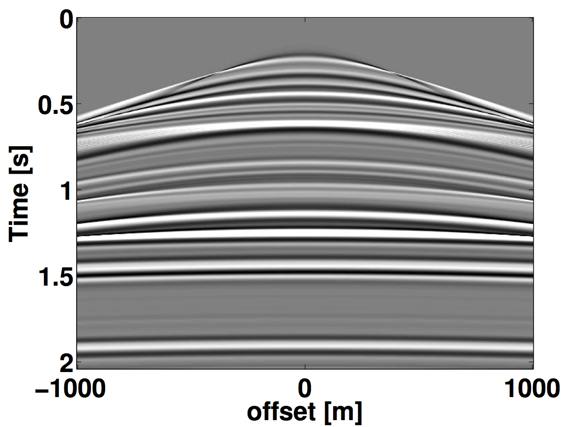
We model a fixed-spread acquisition configuration by simulating densely sampled synthetic time-lapse data comprising a baseline data set and a monitor data set \(\textbf{y}_2\) using \(\textbf{F}\) while keeping the acquisition geometries same . An example of the synthetic seismic data is shown in Figure 1.

In an effort to justify the need to relax time-lapse seismic data acquisition repeatability, we randomly subsample the idealized pre-stack synthetic baseline data by reducing the shot interval, simulating a baseline acquisition with several shots missing at random locations. Similarly, a different randomized subsampling of the monitor data was performed to represent randomized monitor survey with a different set of shot locations missing, independent of the baseline survey.

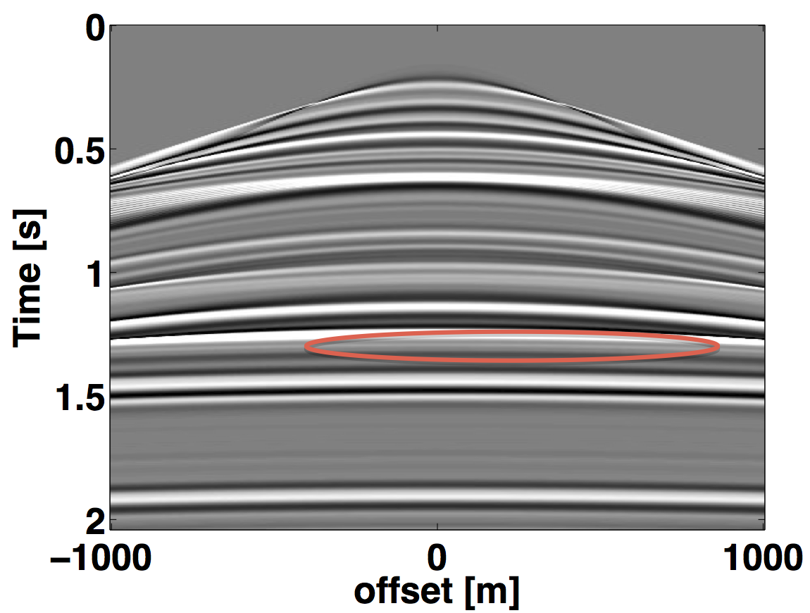
Figure 2 shows an example of the observed common midpoint (CMP) gather indicating missing shots in the data. Although we have only simulated data with missing shots between the vintages, this can equally be extended to missing receivers or missing shots and receivers. This experiment produces time-lapse data from different acquisition geometries, resulting in different sets of shot data and missing traces. In addition, we can also extend this experiment to simultaneous marine acquisition where seismic sources fire at randomly dithered times (Wason & Herrmann, 2013).

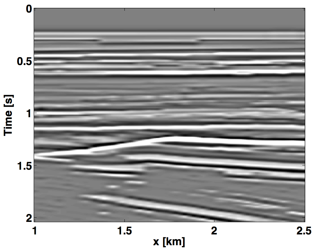
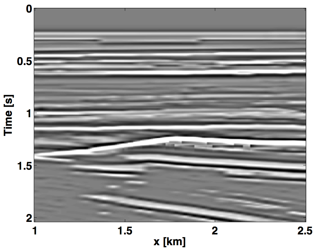
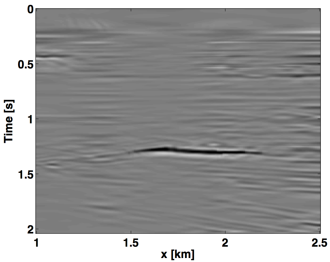
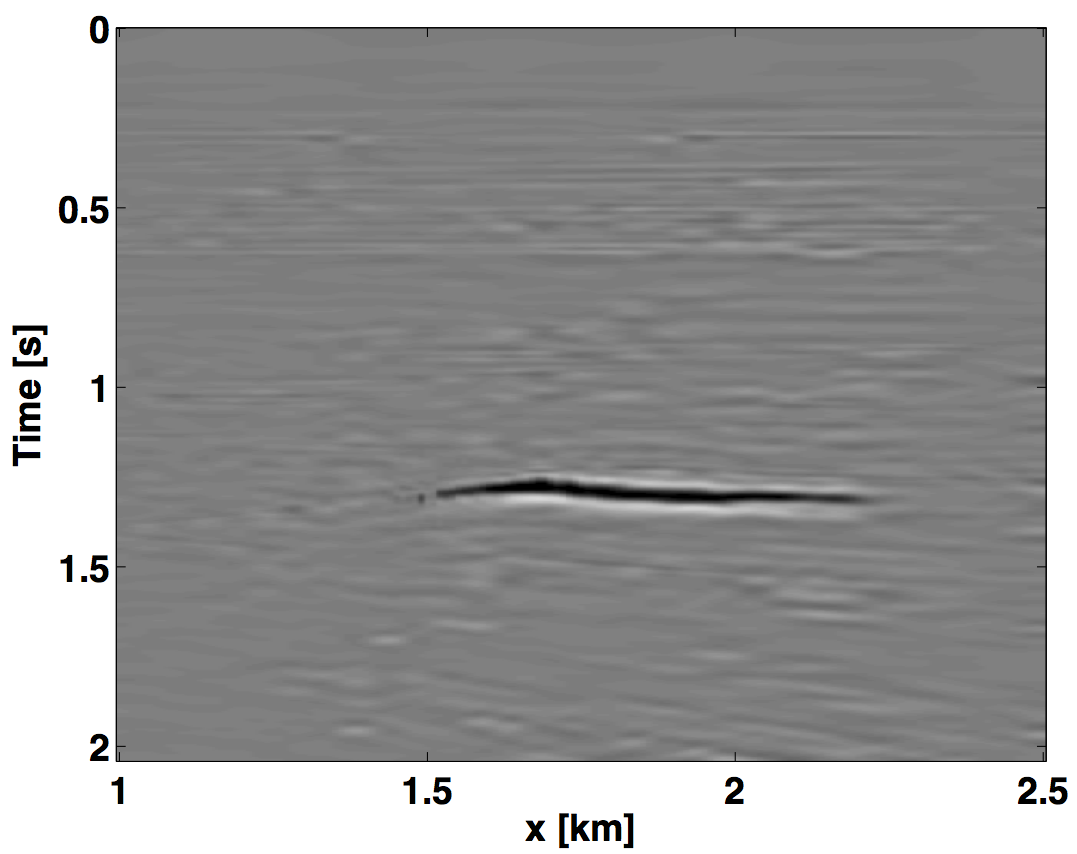
Conventional processing involving NMO and stacking was applied to the densely sampled idealized data sets and this produced a baseline stacked section and monitor stacked section respectively. Figure 3 shows the true (idealized) stacked sections. These served as a benchmark for the rest of our experiment. The stacked section shows the complexity of the model with an indication of strong impedance contrast at different time depths. The time-lapse signal is at a time-depth of between 1.2s and 1.4s and varies laterally over a range of approximately 1km.

To establish the effects of randomized time-lapse survey without repetition and with different subsampling ratios, as it relates to inversion for the stacked sections, we performed experiments for different subsampling ratios. We investigated the inversion results using IRS and JRM, when we have severely subsampled data (1% data) and when the data is less subsampled (5% data). The signal-to-noise ratio (SNR) of our results were also computed, since we know the true time-lapse signal. The inflation of these figures is permissible since we are in an idealized setting and they do illustrate the potential uplift of what happens when the wave propagation effects are completely accounted for or when the physics is right.

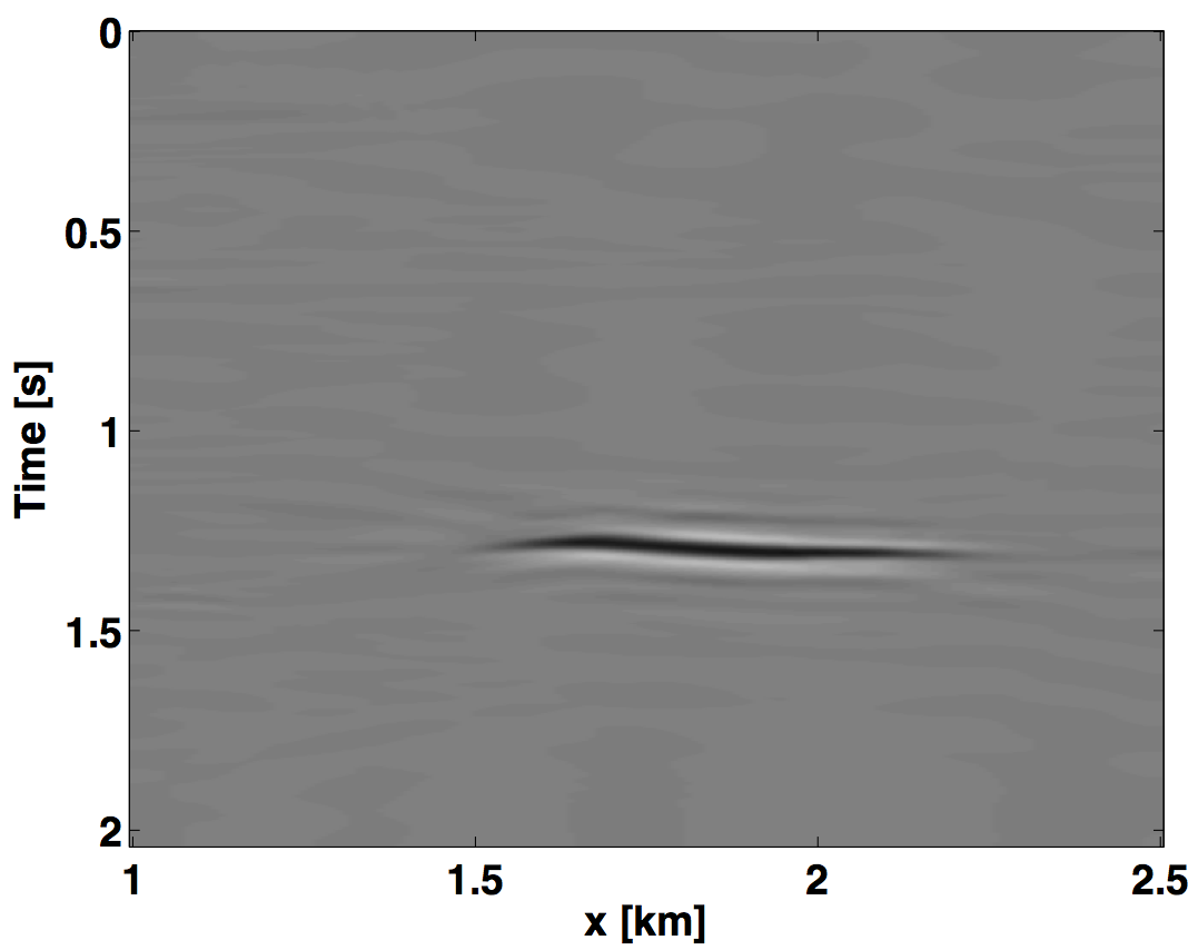
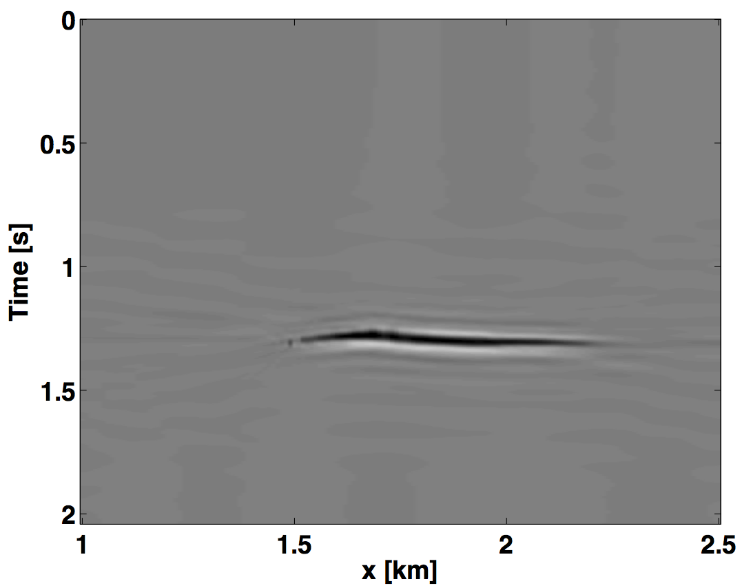
The top row of Figure 4 shows the estimated difference time-lapse stacked sections when the acquired data is just 1% of the idealized densely sampled pre-stack data. In comparison with the ideal stacked sections, we notice a poor match using the IRS (SNR = 0.27dB) and good recovery using the JRM (SNR = 6.28dB). The artifacts observed in the difference stacked sections using the IRS poses a significant problem for interpreters especially when the time-lapse signal is very weak. Such a weak signal will be lost in field data having considerable amount of non-repeatable noise. We have modeled a strong time-lapse signal, so we can still delineate signals from artifacts. We also note that the joint recovery approach benefits more in recovering the 4D difference than the independent recovery strategy. Although not shown here for brevity, we observed that an attempt to recover the full wavefield using the observed data fails considerably regardless of the method employed. However, we expect an improved performance as subsampling ratio decreases.

The next experiment is an inversion for the time-lapse stacked sections using randomly selected 5% of the shots from the densely sampled data, again without repetition. In line with our observation from using 1% of the data, we noticed a significant increase (5.03dB for IRS and 8.36dB for JRM) in the SNR levels of the estimated stacked sections. Consequently, the artifacts level in the difference section is reduced and the resolution of the recovered time-lapse signal is increased as shown in the bottom row of Figure 4. In both subsampling cases, the joint recovery method performs significantly better than the independent recovery method because it exploits the shared information between the observed time-lapse data.

Discussion and Conclusions

The synthetic study is idealistic in that it uses the same forward modeling operator in the inversion scheme. This is necessary for the inversion to be stable, as we require our data to be in the range of the modeling operator. In other words, it is very crucial to account for the physics of the wave propagation in the forward modeling operator. We have also worked with noiseless synthetic data, although we do not expect a poor performace of our methods in such case. Despite our study being idealistic, it is proof of concept of a potential formulation for analysis of 4D signals in the image domain where we have randomized and subsampled measurements from a baseline survey and monitor survey. We have investigated the performance of the recovery algorithms as a function of subsampling ratio and have studied the results for few subsampling ratios . We applied the independent recovery approach and the joint recovery method, and recovered the stacked sections as well as the 4D stacked sections. We observed that extension of our algorithm to recovery of time-lapse stacked section is not as computationally expensive as its application to the recovery of the densely sampled wavefields. In addition, this formulation is not limited to analysis of just two vintages of time-lapse data. It can be applied to multiple time-lapse data which have been acquired with different source/receivers missing.

In conclusion, we have presented an extension of our randomized sampling strategy for time-lapse data acquisition, to estimation of stacked sections. We show that imaging of time-lapse data and stacking are two related phenomena and both follow the same inversion procedure. We present 2D inversion results for a synthetic model illustrating the feasibility of randomized sampling for time-lapse studies, and the results demonstrate the usefulness of the joint recovery method for extracting 4D signals from significantly subsampled time-lapse data. We claim that time-lapse data acquired without repetition, can be processed to obtain stacked sections which reveal high-fidelity 4D difference provided we carry out a sparsity-promoting inversion program. In addition, we distinguish between two recovery algorithms that can both handle the measured data while delineating between the efficiency of the methods when the data are severely and less subsampled. The next step in our study is to extend this methodology to realistic wave equation based inversion of seismic data from time-lapse surveys without repetition, and produce migrated images in depth.

Acknowledgements

This work was financially supported in part by the Natural Sciences and Engineering Research Council of Canada Discovery Grant (RGPIN 261641-06) and the Collaborative Research and Development Grant DNOISE II (CDRP J 375142-08). This research was carried out as part of the SINBAD II project with support from the following organizations: BG Group, BGP, BP, Chevron, ConocoPhillips, CGG, ION GXT, Petrobras, PGS, Statoil, Total SA, WesternGeco, Woodside.

References

Ayeni, G., Tang, Y., Biondi, B., & others. (2009). Joint preconditioned least-squares inversion of simultaneous source time-lapse seismic data sets. In 2009 sEG annual meeting. Society of Exploration Geophysicists.
Baron, D., Duarte, M. F., Sarvotham, S., Wakin, M. B., & Baraniuk, R. G. (2005). An information-theoretic approach to distributed compressed sensing. In Proc. 45rd conference on communication, control, and computing.
Brown, G., & Paulsen, J. (2011). Improved marine 4D repeatability using an automated vessel, source and receiver positioning system. first Break, 29(11), 49–58.
Eggenberger, K., Christie, P., Manen, D.-J. van, & Vassallo, M. (2014). Multisensor streamer recording and its implications for time-lapse seismic and repeatability. The Leading Edge, 33(2), 150–162.
Eiken, O., Haugen, G. U., Schonewille, M., & Duijndam, A. (2003). A proven method for acquiring highly repeatable towed streamer seismic data. Geophysics, 68(4), 1303–1309.
Landrø, M. (1999). Repeatability issues of 3-d vSP data. Geophysics, 64(6), 1673–1679.
Lumley, D., & Behrens, R. (1998). Practical issues of 4D seismic reservoir monitoring: What an engineer needs to know. SPE Reservoir Evaluation & Engineering, 1(6), 528–538.
Oghenekohwo, F., Esser, E., & Herrmann, F. J. (2014, January). Time-lapse seismic without repetition: reaping the benefits from randomized sampling and joint recovery. EAGE. UBC; UBC. Retrieved from https://www.slim.eos.ubc.ca/Publications/Public/Conferences/EAGE/2014/oghenekohwo2014EAGEtls.pdf
Porter-Hirsche, J., & Hirsche, K. (1998). Repeatability study of land data aquisition and processing for time lapse seismic.
Rickett, J., & Lumley, D. (2001). Cross-equalization data processing for time-lapse seismic reservoir monitoring: A case study from the gulf of mexico. Geophysics, 66(4), 1015–1025.
Wason, H., & Herrmann, F. J. (2013, September). Time-jittered ocean bottom seismic acquisition. SEG. Retrieved from https://www.slim.eos.ubc.ca/Publications/Public/Conferences/SEG/2013/wason2013SEGtjo/wason2013SEGtjo.pdf