Randomized HSS acceleration for full-wave-equation depth stepping migration

Lina Miao^*, Polina Zheglova^*, and Felix J. Herrmann^*
*Seismic Laboratory for Imaging and Modeling (SLIM), University of British Columbia

Introduction

Migration methods based on solution of the full wave equation have become the state of the art in modern exploration seismology. They provide the benefits of more accurate imaging in complex geological scenarios with steep dips and overhangs, multipathing and complex overburden. However, imaging methods based on modeling with the full wave equation can be quite expensive for large scale problems, especially in three dimensions. Therefore methods based on depth stepping remain of interest. In such methods, one extrapolates the wavefields in depth rather than extrapolating in time or solving the implicit monochromatic Helmholtz equation. Depth extrapolation is notoriously unstable due to the existence of the evanescent wave components (Wapenaar & Grimbergen, 1998). To handle this instability, several method have been proposed. One of the most promising methods that we are aware of is the method of Sandberg & Beylkin (2009), where they claimed that the spectral projector can filter out the evanescent waves without losing of any propagating wave components. In this work we revisit this method and propose to further improve its computational performance with a recently developed technique – the randomized HSS technique. For simplicity, the methodology and results are presented in two dimensions, but they generalize to three dimensions in a straightforward manner.

Assuming that we are given a survey recorded at a surface \(z_{0}\), the wave propagation can be described by the acoustic wave equation (Sandberg & Beylkin, 2009): \[ \begin{equation} \label{eq:AcousticWaveEquation} \begin{split} p_{tt} = v(z,x)^2(p_{xx} + p_{zz}),\\ p(x,0,t) = 0, t \geq 0,~~~\\ \begin{cases} p(x,z,0) = f(x),\\ p_t(x,z,0) = g(x),\\ \end{cases} \end{split} \end{equation} \] where \(v(x,z)\) is the velocity,\(p(z,x,t)\) is the acoustic pressure at point \((x,z)\), \(f(x)\) is the initial pressure at time \(0\), and the subscripts indicate partial derivatives. Applying the Fourier transform with respect to time to Equation \(\eqref{eq:AcousticWaveEquation}\) and rearranging, we obtain the following equation for \(\hat{p}\): \[ \begin{equation} \label{eq:hatpzz} \hat{p}_{zz} = \left [ -\left(\frac{ \omega}{v(x,z)} \right)^2 - D_{xx} \right]\hat{p} := L\hat{p}. \end{equation} \] Here \(L\) is the operator in the square brackets. We consider Equation \(\eqref{eq:hatpzz}\) with the initial conditions \(q\) and \(q_z\) at the surface \(z = z_0\): \[ \begin{equation} \label{eq:initialvalueproblem} \begin{cases} \hat{p}(x,z_0,\omega) = \hat{q}(x,z_0,\omega)\\ \hat{p}_z(x,z_0,\omega) = \hat{q}_z(x,z_0,\omega) \end{cases} \end{equation} \] where in practice, \(\hat{q}\) and \(\hat{q}_z\) stand for the wavefield specified at the surface \(z = z_0\) and its first derivative along \(z\) direction respectively.

A first order depth stepping scheme can be formulated based on the initial-value problem formed by Equations \(\eqref{eq:hatpzz}\) and \(\eqref{eq:initialvalueproblem}\) (Sandberg & Beylkin, 2009): \[ \begin{equation} \label{eq:depthextrapolation} \begin{aligned} \frac{d}{dz} \begin{bmatrix} \hat{p} \\ \hat{p}_z \end{bmatrix} = \begin{bmatrix} 0&1 \\ L&0\end{bmatrix} \begin{bmatrix} \hat{p}\\ \hat{p}_z \end{bmatrix}. \end{aligned} \end{equation} \] However, this depth stepping scheme is unstable. The cause of this instability is the indefinite nature of the self-adjoint operator \(L\), such that the positive eigenvalues will result in exponential growth of the wavefield during depth extrapolation. Physically, the negative eigenvalues correspond to propagating wave modes, and the positive eigenvalues are associated with the evanescent wave modes. The evanescent wave modes can be suppressed by zeroing out the positive eigenvalues via the eigenvalue decomposition of the operator \(L\), however, the eigenvalue decomposition is too expensive to be practical in large scale seismic imaging problems. Alternatively, the spectral projector provides an eigenvalue decomposition free approach to stabilize the extrapolation operator.

Stable depth extrapolation with spectral projector

The mathematical background of the spectral projector can be found in the survey of Kenney & Laub (1995), where a projector \(\mathcal{P}\) projecting onto the non-positive invariant subspace of a self-adjoint matrix \(L\) is defined as: \[ \begin{equation} \label{eq:2_8} \mathcal{P} = (I - \text{sign}(L))/2 . \end{equation} \] Here \(I\) stands for the identity matrix, and \(\text{sign}(L)\) stands for the matrix sign function of the matrix \(L\). In other words, with the spectral projector \(\mathcal{P}\) applied to the unstable extrapolator \(L\), one obtains a stabilized extrapolation operator \(\mathcal{P}L\mathcal{P}\) that suppresses the evanescent wavefield modes associated with the positive eigenvalues of \(L\) during the extrapolation. Compared to other approximate Fourier filtering techniques (e.g. Kosloff & Baysal, 1983), the spectral projector only removes the true evanescent waves (associated with the positive eigenvalues) without relying on the assumption that the medium is locally laterally invariant.

The computation of the spectral projector \(\mathcal{P}\) relies on the computation of the matrix sign function: \(\text{sign}(L)\). Recall that the matrix sign function of the self adjoint matrix \(L\) can be written as: \[ \begin{equation} \label{eq:signv} \text{sign}(L) = V\text{sign}(\Lambda)V^*, \end{equation} \] where \(V\) contains the eigenvectors of \(L\), and \(\Lambda\) is the diagonal matrix of the eigenvalues of \(L\).

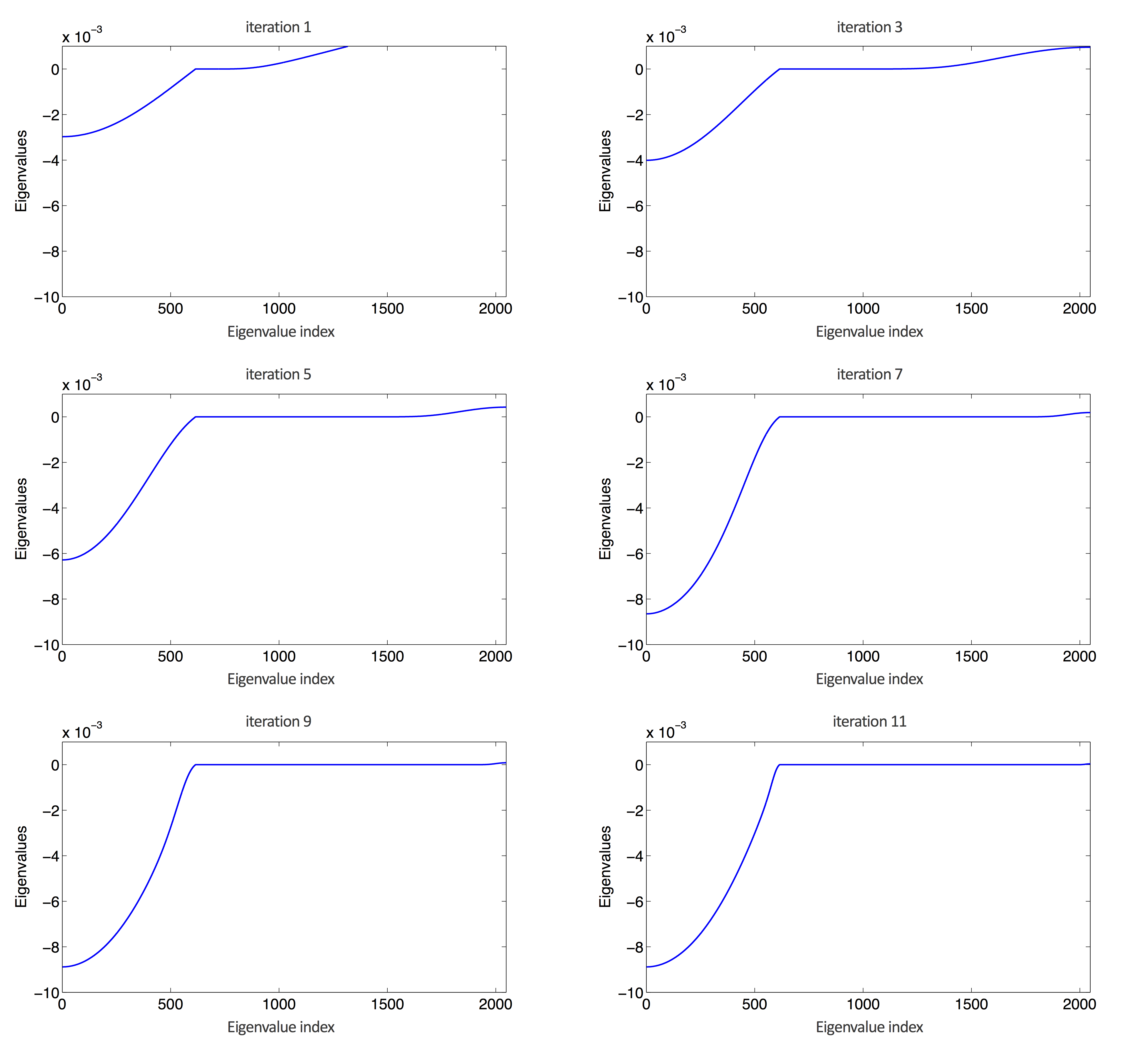
Auslander & Tsao (1991) introduced the Newton - Schulz method to compute the matrix sign function without eigenvalue decomposition. The Newton-Schulz iteration (Algorithm 1) converges to the matrix sign function using a matrix polynomial recursion with a quadratic convergence rate. Figure 1 illustrates the eigenvalues of the operator \(\mathcal{P}L\mathcal{P}\) computed with Algorithm 1 and Equation \(\eqref{eq:2_8}\). It is clear from Figure 1 that the positive eigenvalues converge to zeros in just a few iterations, while the non-positive eigenvalues remain intact.

Input: Self adjoint matrix \(L\)
Output: \(S:=\text{sign}(L)\)
1. Initialize \(S_0 = L/||L||_2\), where \(||L||_2\) stands for the 2 norm of matrix \(L\).
2. For \(k = 1...N\),   \(S_{k+1} = \frac{3}{2} S_k - \frac{1}{2}S_k^3\)

Efficient computation of the spectral projector with randomized HSS technique}

Even though the Newton-Schulz iteration (Algorithm 1) can compute the matrix sign function in an affordable number of polynomial iterations, we need to address the computationally intensive part in it: the matrix-matrix multiplication. Even if we start with a sparse matrix, the matrices involved in the recursion fill up quickly in early iterations. The \(\mathcal{O}{(n^3)}\) computational complexity for dense matrix-matrix multiplication is not practical for any realistic seismic problem, especially in 3D, where the matrix size can be of order \(10^6\) by \(10^6\) or larger. Therefore we need a powerful engine for fast matrix-matrix multiplication in order to compute the spectral projector efficiently. For this purpose, in this section we propose an efficient acceleration with the randomized Hierarchically Semi-Separable (HSS) method.

HSS matrix representation was introduced as an alternative way of representing a particular class of in general dense \(n \times n\) matrices. The literature on HSS representation is numerous, for more information the reader is referred to (e.g. S. Chandrasekaran et al., 2006; Sheng, Dewilde, & Chandrasekaran, 2007; Xia, 2012), and references therein. Instead of using the \(n^2\) entires of a matrix, the HSS representation exploits the low rank structure of its particular sub-matrices. The HSS matrix representation has a nice property of linear complexity of matrix computations and storage with respect to the matrix size. With regards to the matrix-matrix multiplication, the cubic complexity \(\mathcal{O}{(n^3)}\) for ordinary dense matrices is reduced to linear (\(\mathcal{O}{(nk^3)}\)) complexity via HSS matrix representation, where \(n\) is the matrix size, and \(k\) is the maximum rank of the transition matrices in the HSS tree (W. Lyons, 2005).

Further improvement in efficiency of the HSS algorithms can be achieved by making use of the recently developed randomized singular value decomposition (rSVD) algorithm. In many HSS algorithms, especially during the process of constructing HSS representations, SVDs (or other rank revealing algorithms) are recursively used in compressing the low rank off-diagonal components. The rSVD algorithm (Tygert & Rokhlin, 2007) is one of those algorithms (Halko, Martinsson, & Tropp, 2011) that compute fast matrix factorizations by exploiting the random probing technique. In rSVD, random probing is used to identify the compressed subspace that captures most of the action of a matrix, and then further matrix manipulations are applied to compute the approximate SVD result. In this work, we implement the rSVD algorithm proposed by Tygert & Rokhlin (2007), and incorporate the rSVD algorithm into the standard HSS algorithms, generating more efficient randomized HSS algorithms. Tygert & Rokhlin (2007) claim the rSVD algorithm to have numerical complexity of \(\mathcal{O}{(k^2(m+n))}\) with a small constant number for a rank \(k\) \(m\times n\) matrix, where \(k \leq n \leq m\).

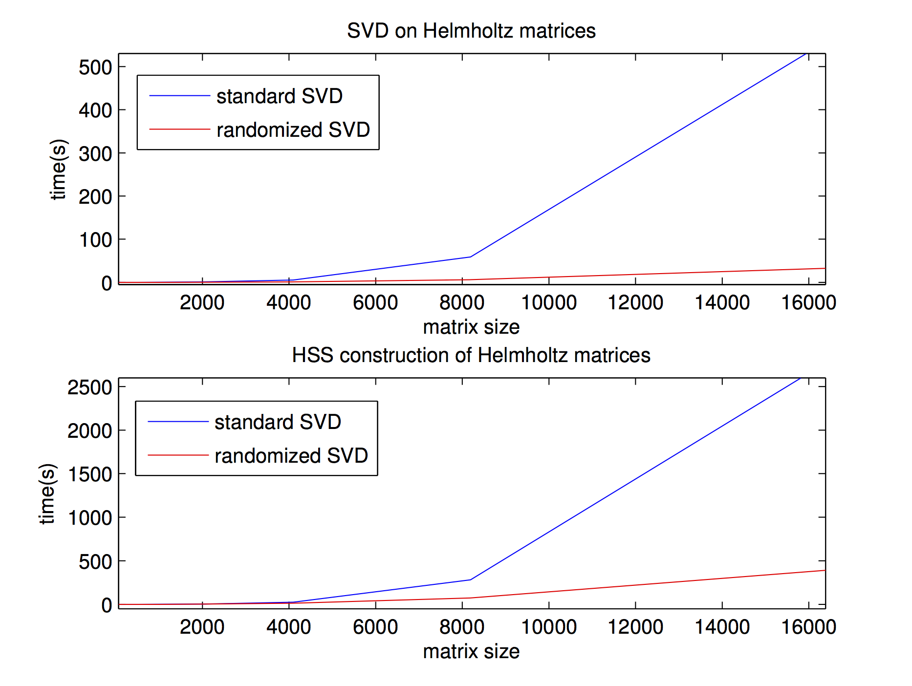
Below, we show the time improvement achieved with the randomized HSS method in comparison with the standard HSS method in HSS tree structure construction (using MATLAB built-in SVD’s). Figure 2 shows computational performance of the randomized SVD algorithm and the randomized HSS construction with the error controlled to the level of 1e-6. The first plot shows an SVD and rSVD comparison on a series of depth extrapolation matrices \(L\) of different sizes. The second plot shows a comparison of HSS construction using standard SVD and rSVD. Some general conclusions can be drawn from those two plots: first, the rSVD algorithm significantly decreases the computational time compared to the standard SVD algorithm; second, randomized HSS construction time is also significantly reduced compared to the standard SVD algorithm, and the advantage becomes more distinct as the matrix size grows. For other HSS operations, the improvement from the randomized HSS would be determined according to how intensively SVD’s are used by specific algorithms.

In Figure 3 we show the computational cost of the spectral projector computed with the eigenvalue decomposition (blue line), the polynomial recursion using ordinary matrix-matrix multiplication (black line), and the randomized HSS acceleration (red line) for different matrix sizes. As the matrix size grows, the time advantage of randomized HSS acceleration starts to be obvious.

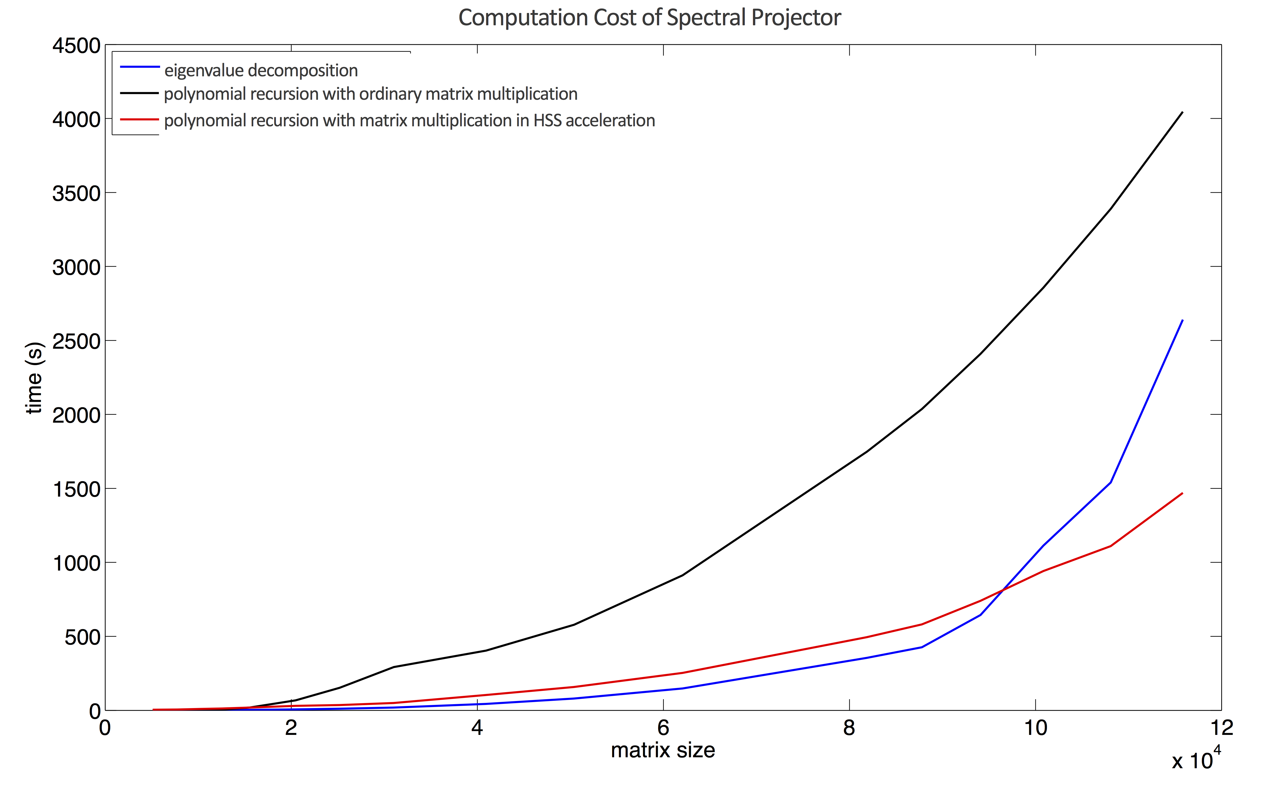
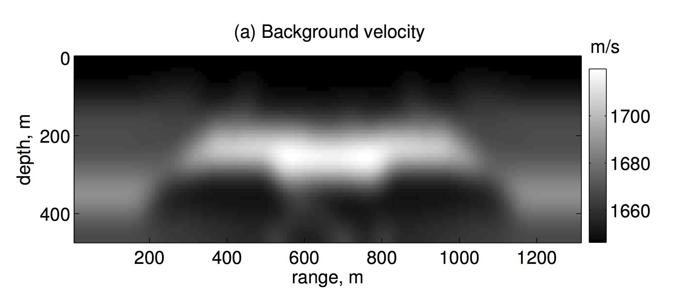
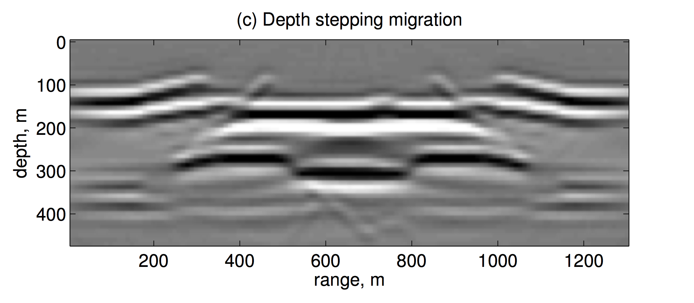
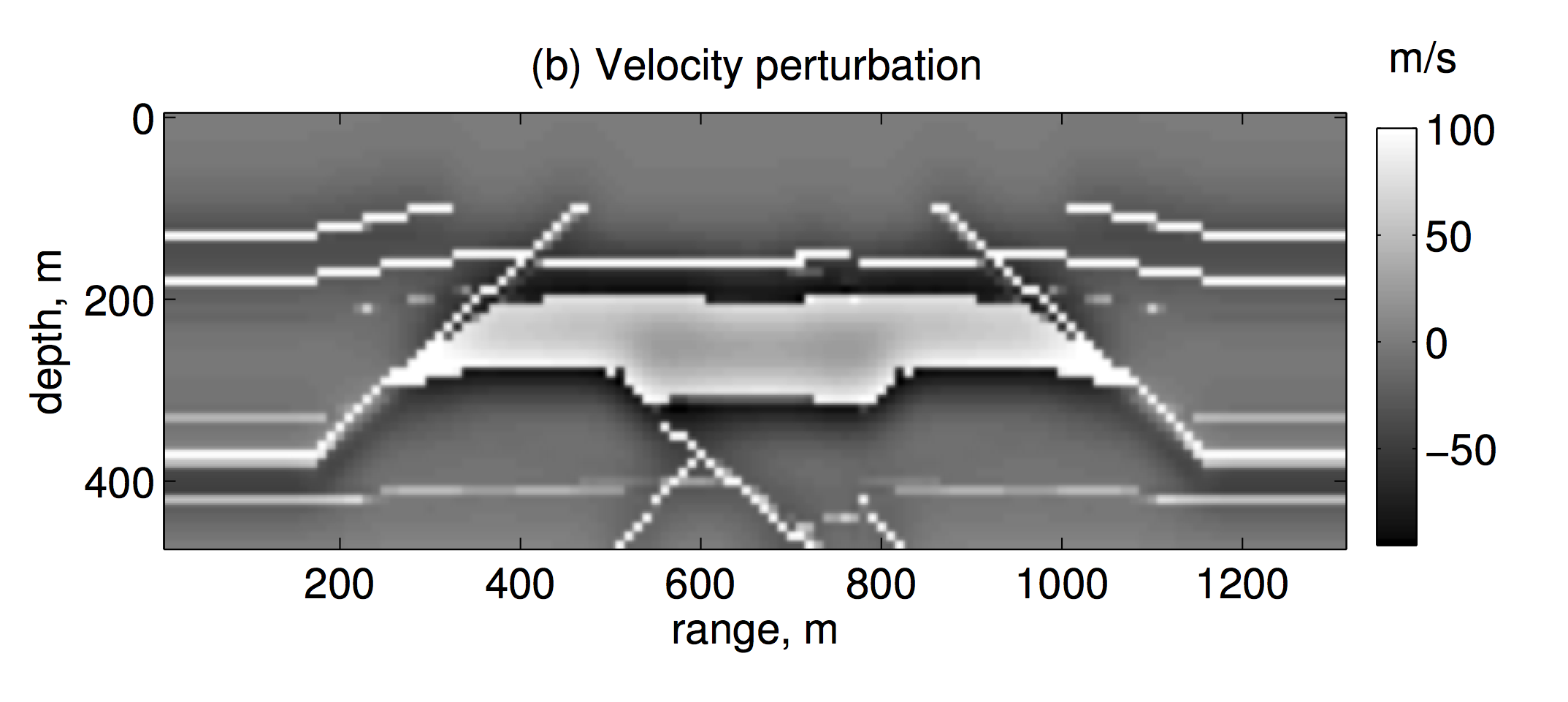
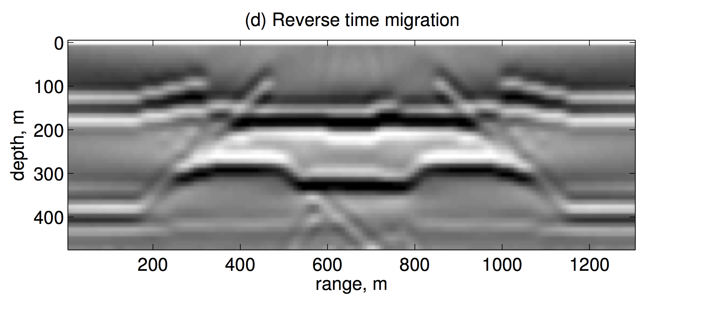
Figure 4 shows a migration example with the laterally varying background velocity model, plot (a), and the model perturbation, plot (b). The density is assumed constant. The grid spacing is 10 m in both horizontal and vertical direction. In this experiment, we model the frequency range of 5 Hz to 35 Hz using the linearized constant-density acoustic frequency-domain modeling operator. The computational domain in which modeling and migration is performed is wider than the part shown in Figure 4(a-d), since a horizontal taper was applied to the wavefield at the left and right boundary to suppress the wrap around of the wavefield from the periodic boundary conditions during depth extrapolation. Sources and receivers were put on the top layer of grid points of the wider domain. Figure 4(c) shows the imaging result with two-way wave equation depth stepping migration algorithm of Sandberg & Beylkin (2009) with the proposed randomized HSS acceleration. Although the result of the depth stepping migration is essentially clean with no significant artifacts, we filtered it using 1st order finite differences in the vertical direction to enhance the perturbation. Figure 4(d) shows reverse time migration (RTM) result. The RTM result was filtered using 2nd order finite differences in the vertical direction to suppress the low frequency artifacts. The images are comparable in quality, except for the area under the salt body and the thin slanting reflectors close to the boundaries of the domain.

Conclusion

In this work we proposed a randomized HSS acceleration for the full wave equation depth-stepping migration method first introduced by Sandberg & Beylkin (2009). Specifically, the rSVD technique is used to speed up the HSS matrix operations utilized in the computation of the spectral projector of the depth-stepping operator. Tests with the randomized HSS acceleration technique demonstrate its efficiency compared to conventional techniques, and the advantage becomes more apparent as the problem size grows. The tests were performed in two dimensions, but extension to 3D is straightforward. The randomized HSS accelerated depth-stepping full wave equation migration can be an efficient alternative to RTM.

Acknowledgements

This work was financially supported in part by the Natural Sciences and Engineering Research Council of Canada Discovery Grant (RGPIN 261641-06) and the Collaborative Research and Development Grant DNOISE II (CDRP J 375142-08). This research was carried out as part of the SINBAD II project with support from the following organizations: BG Group, BGP, BP, Chevron, ConocoPhillips, CGG, ION GXT, Petrobras, PGS, Statoil, Total SA, WesternGeco, Woodside.

References

Auslander, L., & Tsao, A. (1991). On parallelizable eigensolvers. Citeseer.
Chandrasekaran, S., Dewilde, P., Gu, M., Lyons, W., & Pals, T. (2006). A fast solver for hSS representations via sparse matrices. SIAM Journal on Matrix Analysis and Applications, 29(1), 67–81.
Halko, N., Martinsson, P.-G., & Tropp, J. A. (2011). Finding structure with randomness: Probabilistic algorithms for constructing approximate matrix decompositions. SIAM Review, 53(2), 217–288.
Kenney, C. S., & Laub, A. J. (1995). The matrix sign function. Automatic Control, IEEE Transactions on, 40(8), 1330–1348.
Kosloff, D. D., & Baysal, E. (1983). Migration with the full acoustic wave equation. Geophysics, 48(6), 677–687.
Lyons, W. (2005). Fast algorithms with applications to pDEs (PhD thesis). UNIVERSITY of CALIFORNIA.
Sandberg, K., & Beylkin, G. (2009). Full-wave-equation depth extrapolation for migration. Geophysics, 74(6), WCA121–WCA128.
Sheng, Z., Dewilde, P., & Chandrasekaran, S. (2007). Algorithms to solve hierarchically semi-separable systems. Operator Theory: Advances and Applications, 176, 255–294.
Tygert, M., & Rokhlin. (2007). A randomized algorithm for approximating the sVD of a matrix. Retrieved from https://www.ipam.ucla.edu/publications/setut/setut_7373.pdf
Wapenaar, K., & Grimbergen, J. L. (1998). A discussion on stability analysis of wave field depth extrapolation. In 1998 sEG annual meeting.
Xia, J. (2012). On the complexity of some hierarchical structured matrix algorithms. SIAM Journal on Matrix Analysis and Applications, 33(2), 388–410.