Mitigating data gaps in the estimation of primaries by sparse inversion without data reconstruction

Introduction

Multiple removal is a crucial aspect of seismic signal processing that constantly face a difficult quad-lemma between accuracy, robustness, low computational complexity, and full-azimuthal sampling. Current prediction-subtraction methods such as Surface-Related Multiple Removal (Verschuur, 1992) face limits in accuracy and robustness when confronted with undersampled data of limited quality, prompting recent developments in whole- wavefield inversion/deconvolution techniques to decrease dependence on practitioner guesswork and QC. In recent work Tim T Y Lin & Herrmann (2014) proposed a multiscale strategy that reduces the computational burden by using coarser spatial sampling grids while exploiting the unique way in which REPSI (Tim T. Y. Lin & Herrmann, 2013) mitigates spatial aliasing. While this approach successfully addressed some of the computational costs associated with ``data-driven’’ techniques typified by the Raleigh-Helmholtz reciprocity relationship between the field-measured wavefield data and its multiple-free version (Fokkema & Berg, 1993; Frijlink, Borselen, & Söllner, 2011), these methods all rely on dense wide-azimuthal samplings that include near offset information.

This reliance on dense samplings has and continues to be challenging and has called for intricate on-the-fly trace interpolations as part of SRME predictions or extensions of EPSI to include missing data as unknowns (Groenestijn & Verschuur, 2009), forcing the algorithm to alternate between estimating the source, the surface-free Green’s function and this missing data. While the initial results of the latter technique in EPSI has been successful, these explicit inversion schemes do not exploit possibilities to extend the multiple-prediction operator to include recursive terms that model the imprint on missing data. Our main contribution in this work is to come up with a formulation where the effects of missing data–i.e., a mask acting on the data matrix zeroing entries where data is missing, are incorporated in the forward model of EPSI explicitly through auto-convolution terms.

Our work is organized as follows. First, we briefly summarize the EPSI formulation as an alternating optimization problem inverting for the source and surface-free Green’s by promoting sparsity via the \(\ell_1\)-norm on the latter. We make the dependence of EPSI on the fully sampled upward going wavefield explicit to emphasize the dependence of the formulation on dense sampling. Next, we discuss the method proposed by Groenestijn & Verschuur (2009), which extends EPSI to the situation where information on the upgoing wavefield is missing, followed by our method where we incorporate convolutional terms in the forward modeling operator that account for missing (e.g., near offsets) traces in the upgoing wavefield. The different terms in these expansion predict the impact of missing data on the prediction of first and higher multiples. We conclude by demonstrating the efficacy of this method on both synthetic and field data sets.

Theory

The basic assumption of surface-related multiple removal with EPSI is that, with noiseless and perfectly sampled up-going seismic wavefield \(\vec{P}\) at the Earth’s surface (with seismic reflectivity operator \(\vec{R}\), typically close to \(\vec{-I}\)) due to a finite energy source wavefield \(\vec{Q}\), there exists an operator \(\vec{G}\) for every frequency in the seismic bandwidth such that the relation \(\vec{P} = \vec{G}\vec{Q} + \vec{R}\vec{G}\vec{P}\) holds true. Here we use the “detail-hiding” notation (Berkhout & Pao, 1982) where all upper-case bold quantities are monochromatic data-matrices, with the row index corresponding to the discretized receiver positions and column index the source positions. Moreover, \(\vec{G}\) is interpreted as the (surface) multiple-free subsurface Green’s function. The term \(\vec{GQ}\) is interpreted as the primary wavefield, while the term \(\vec{R}\vec{G}\vec{P}\) contains all surface-related multiples.

Since only \(\vec{P}\) can be measured, inverting the above relation for \(\vec{GQ}\) admits non-unique solutions without additional regularization. Based on the argument that a discretized physical representation of \(\vec{G}\) resemble a wavefield with impulsive wavefronts, the Robust EPSI algorithm (REPSI, Tim T. Y. Lin & Herrmann, 2013) attempts to find the sparsest possible \(\vec{g}\) in the physical domain (from here on, all lower-case symbols indicate discretized physical representations of previously defined quantities). Specifically, it solves the following optimization problem in the space-time domain: \[ \begin{gather} \label{eq:EPSIopt} \min_{\vector{g},\;\vector{q}}\|\vector{g}\|_1 \quad\text{subject to}\quad f(\vec{g},\vec{q};\vec{p}) \le \sigma,\\ \nonumber f(\vec{g},\vec{q};\vec{p}) := \|\vector{p} - M(\vector{g},\vector{q};\vector{p})\|_2, \end{gather} \] where the forward-modeling function \(M\) can be written in terms of the data-matrix notation \(M(\vector{G},\vector{Q};\vector{P}) := \vec{G}\vec{Q} + \vec{R}\vec{G}\vec{P}\). Problem \(\eqref{eq:EPSIopt}\) essentially asks for the sparsest (via minimizing the \(\ell_1\)-norm) multiple-free impulse response that explains the surface multiples in \(\vector{p}\), while ignoring some amount of noise as determined by \(\sigma\).

To consider the parts of data \(\vec{P}\) that are not sampled, we now introduce a masking matrix \(\vec{K}\) that is has same dimensions as the data-matrices. The elements of mask \(\vec{K}\) has value 0 where we do not have data at the corresponding source-receiver position pair, and the value 1 at sampled positions. Thus, we can segregate parts of the data that are sampled as \(\vec{P'} := \vec{K}\circ\vec{P}\), where the symbol \(\circ\) denotes the matrix Hadamard product. Similarly, we introduce the complement mask \(\vec{K_c}\) (a “stencil”), such that the unknown parts of the data can be written as \(\vec{P''} := \vec{K_c}\circ\vec{P}\) with \(\vec{P'}+\vec{P''}=\vec{P}\). The presence of these gaps are a significant source of error in the calculation of \(M\) (see, for example, Verschuur, 2006).

Explicit data inversion

As first proposed by Groenestijn & Verschuur (2009), we can augment the optimization problem \(\eqref{eq:EPSIopt}\) to explicitly reconstruct \(\vec{p''}\) from intermediate estimates of \(\vec{g}\) such that the accuracy of \(M\) can be improved as the algorithm converges. We now overload the definition of \(M\) with a more general modeling operator \[ \begin{equation} \label{eq:normal_modeling} M(\vector{G},\vector{Q},\vector{P''};\vector{P'}) := \vec{G}\vec{Q} + \vec{R}\vec{G}(\vec{P'} + \vec{P''}), \end{equation} \] which defines a more complicated inversion problem that has \(\vec{p''}\) as an inversion variable \[ \begin{gather} \label{eq:EPSIopt_uP} \min_{\vector{g},\;\vector{q},\;\vector{p''}}\|\vector{g}\|_1 \quad\text{subject to}\quad f(\vec{g},\vec{q},\vec{p''};\vec{p'}) \le \sigma,\\ \nonumber f(\vec{g},\vec{q},\vec{p''};\vec{p'}) := \|\vector{p'} + \vec{p''} - M(\vector{g},\vector{q},\vector{p''};\vec{p'})\|_2. \end{gather} \] A major pitfall in solving \(\eqref{eq:EPSIopt_uP}\) via an alternating optimization strategy (or cyclic coordinate descent) is that \(\vec{g}\) and \(\vec{p''}\) are in fact tightly coupled, because we can write the cyclic relation \[ \begin{equation} \label{eq:uP_recursive} \vec{P''} = \vec{K_c}\circ\vec{P} = \vec{K_c}\circ\big[\vec{GQ} + \vec{RGP'} + \vec{RGP''}\big] \end{equation} \] where it is evident that \(\vec{P''}\) can be almost completely characterized by \(\vec{G}\). We therefore would expect that \(\partial\vec{p''}/\partial\vec{g}\) and \(\partial\vec{g}/\partial\vec{p''}\) cannot be ignored when updating \(\vec{p''}\) and \(\vec{g}\). However, while \(\partial\vec{p''}/\partial\vec{g}\) is straightforward to compute, the term \(\partial\vec{g}/\partial\vec{p''}\) is convoluted and necessarily involves \(\vec{Q}^{-1}\) (deconvolving the source function \(\vec{q}\)). Motivated by this observation, we propose to remove \(\vec{p''}\) as an inversion variable all-together, and instead model its multiple contribution with terms that ultimately involve auto-convolutions of \(\vec{g}\).

Alternative: inclusion of auto-convolution terms

Substituting expression \(\eqref{eq:uP_recursive}\) recursively into \(\eqref{eq:normal_modeling}\) results in a new forward-modeling operator into the range of observed data locations with infinitely many terms in a series expansion \[ \begin{align} \nonumber \widetilde{M}(\vec{G},\vec{Q};\vec{P'}) =& \vec{K}\circ\big[\vec{GQ} + \vec{RGP'}\\ \label{eq:1stTerm} & +\;\vec{RGK_c}\circ(\vec{GQ} + \vec{RGP'})\\ \label{eq:2ndTerm} & +\;\vec{RGK_c}\circ\left(\vec{RGK_c}\circ(\vec{GQ} + \vec{RGP'})\right)\\ \nonumber & +\;\Order(\vec{G}^4)\big]\\ \label{eq:inftySeries} :=& \vec{K}\circ\sum_{n=0}^{\infty}\left(\vec{RGK_c}\circ\right)^n \left(\vec{GQ+RGP'}\right). \end{align} \] In this expression we slightly abuse the notation and write matrix Hadamard products as linear operators (valid as long as the corresponding rules of associativity are obeyed). Since high-order multiple decay, we know from physical arguments that \(\|\vec{G}\| < 1\), and therefore \(\eqref{eq:inftySeries}\) converges to \(\vec{K}\circ\left(\vec{I - RGK_c}\circ\right)^{-1} \left(\vec{GQ+RGP'}\right)\). In a noise-free setting with perfect data sampling outside of the holes, we expect \(\widetilde{M}(\vec{G},\vec{Q};\vec{P'})\) to exactly match the observed data \(\vec{P'} = \vec{K}\circ\vec{P}\). Thus we have the following relation: \[ \begin{equation} \label{eq:autoconvSum} \vec{K}\circ\vec{P} = \vec{K}\circ\left(\vec{I - RGK_c}\circ\right)^{-1} \left(\vec{GQ+RGP'}\right). \end{equation} \] The physical interpretation of expression \(\eqref{eq:autoconvSum}\) is clear: if we have access to the total data \(\vec{P}\), we can exactly derive the multiple contribution due to \(\vec{P''}\) by \(\vec{RGK_c}\circ\vec{P}=\vec{RGP''}\). Since \((\vec{K}\circ)^{-1}\) and \((\vec{K_c}\circ)^{-1}\) does not exist, expression \(\eqref{eq:autoconvSum}\) cannot be directly turned into a practical inversion problem. However, it does serve to validate our new forward model \(\widetilde{M}(\vec{G},\vec{Q};\vec{P'})\).

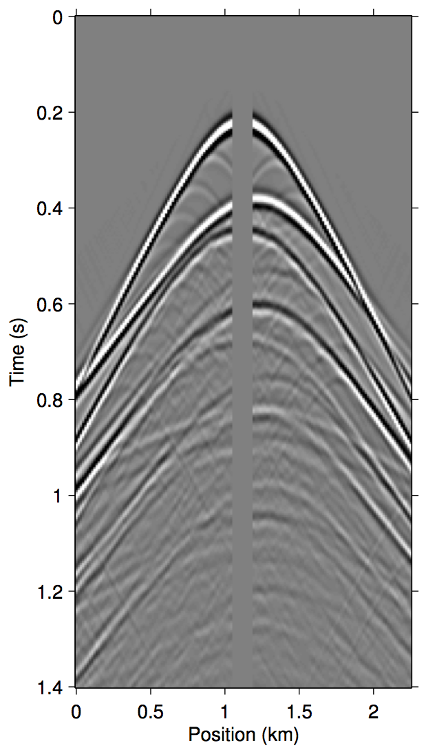
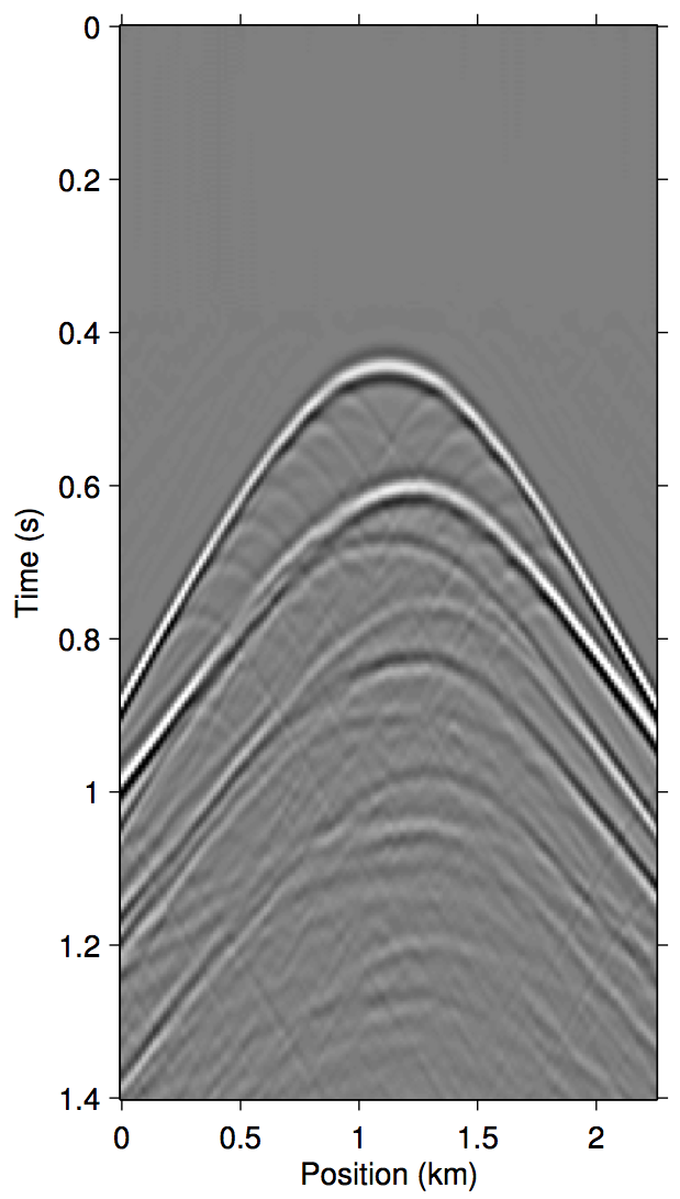
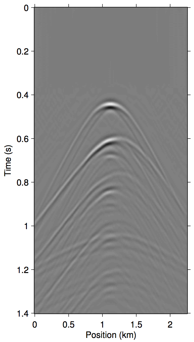
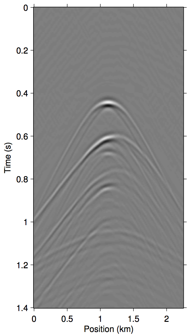
To invert this operator, we propose to invert an approximate \(\widetilde{M}(\vec{G},\vec{Q};\vec{P'})\) that only includes the first few terms of \(\eqref{eq:inftySeries}\). Figure 1 demonstrates a justification of this approach with shot-gather representations of the different terms in \(\eqref{eq:inftySeries}\) for a synthetic dataset with missing near-offset traces (up to 75 m). Comparing panels (d) and (g), it is evident that just the first three terms of \(\eqref{eq:inftySeries}\) is enough to model most of the significant multiple contributions from the missing data \(\vec{p''}\).

Algorithms

With the new forward-modeling operator \(\widetilde{M}(\vec{G},\vec{Q};\vec{P'})\) we can again redefine a new optimization problem based on \(\eqref{eq:EPSIopt_uP}\): \[ \begin{gather} \label{eq:EPSIopt_autoconv} \min_{\vector{g},\;\vector{q}}\|\vector{g}\|_1 \quad\text{subject to}\quad f(\vec{g},\vec{q};\vec{p'}) \le \sigma,\\ \nonumber f(\vec{g},\vec{q};\vec{p'}) := \|\vector{p'} - \widetilde{M}(\vector{g},\vector{q};\vec{p'})\|_2. \end{gather} \] Compared to the EPSI problem with fully-sampled data \(\eqref{eq:EPSIopt}\), the new problem \(\eqref{eq:EPSIopt_autoconv}\) is no longer a linear misfit problem in terms of \(\vec{g}\). In Tim T. Y. Lin & Herrmann (2013), we relied on the bilinear property of \(f(\vec{g},\vec{q};\vec{p'})\) in terms of \(\vec{g}\) and \(\vec{q}\) in order to solve problem \(\eqref{eq:EPSIopt}\). Below we will discuss two possible approaches to modify our solution strategy to account for the additional non-linear auto-convolution terms in \(\widetilde{M}(\vec{G},\vec{Q};\vec{P'})\).

Modified Gauss-Newton

Several existing works on regularized inversion of auto-convolution functions rely on either the Gauss-Newton method or more generally the Levenberg-Marquardt method (Fleischer & Hofmann, 1996; Fleischer, Gorenflo, & Hofmann, 1999). In the same vein, we can adopt a modified Gauss-Newton method introduced in Li, Aravkin, Leeuwen, & Herrmann (2012) to heuristically obtain sparse solutions to \(\eqref{eq:EPSIopt_autoconv}\).

The crux of this approach is to always ensure that the model updates \(\Delta\vec{g}\) are the sparsest possible for any given amount of decrease in \(f(\vec{g},\vec{q};\vec{p'})\). This is achieved most effectively by taking as updates the solution to a Lasso problem (Tibshirani, 1996) around the current Jacobian: \[ \begin{equation} \label{lasso_mGN} \Delta\vec{g}_{k+1} = \mathop{\mathrm{argmin}}_{\vec{g}} \nabla \widetilde{M}_{g_{k}} \vector{g}\quad\text{s.t.}\quad\|\vector{g}\|_1 \le \tau_k, \end{equation} \] where \(k\) is the Gauss-Newton iteration count, and \(\tau_k\) is an iteration-dependent \(\ell_1\)-norm constraint determined in closed-form from the Pareto curve associated with \(\eqref{lasso_mGN}\) (c.f. line 5 of Algorithm 1 in Li et al., 2012). Although this method does not claim to solve \(\eqref{eq:EPSIopt_autoconv}\) exactly, it has been demonstrated to work well at giving sparse solutions to non-linear problems such as full-waveform inversion.

Re-linearization

Another heuristical method is to adapt the same approach used in Tim T. Y. Lin & Herrmann (2013) for the fully-sampled EPSI problem by simply re-linearizing the forward modeling operator at each iteration of the REPSI algorithm (c.f. line 9 of Algorithm 1 in Tim T. Y. Lin & Herrmann, 2013) by \[ \begin{equation*} \begin{aligned} \widetilde{M}_{\vec{G}_k}(\vec{G}) =& \vec{K}\circ\big[\vec{G}\vec{Q}_k + \vec{RGP'} \\ & +\;\vec{RG}_k\vec{K_c}\circ(\vec{G}\vec{Q}_k + \vec{RGP'}) + \;...\big]. \end{aligned} \end{equation*} \] Compared to the modified Gauss-Newton, this approach avoids computing the action of the Jacobian of \(f(\vec{g},\vec{q};\vec{p'})\), which saves the computational cost of one wavefield convolution per term used in \(\widetilde{M}(\vec{G},\vec{Q};\vec{P'})\). As we see below in numerical experiments on real data, the two approaches gives comparable performance, and both approaches outperform pre-EPSI interpolation by parabolic Radon.

Experiments

We now demonstrate the effectiveness of the auto-convolution based problem using a shallow-water marine dataset with 100 m of missing near-offset data. The data has been pre-processed via up-down decomposition to be the upgoing wavefield, and a 3D-to-2D correction of \(\sqrt{t}\) has been applied to the data.

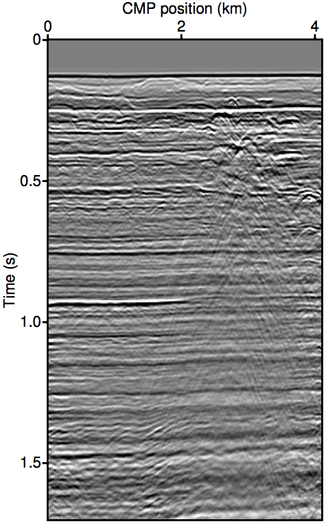
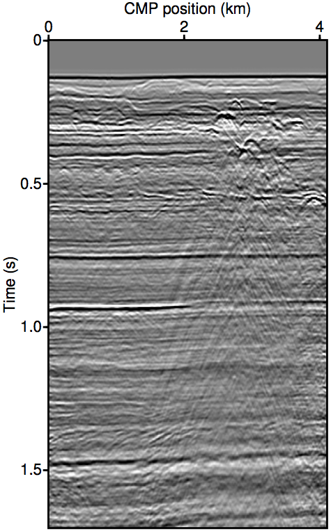
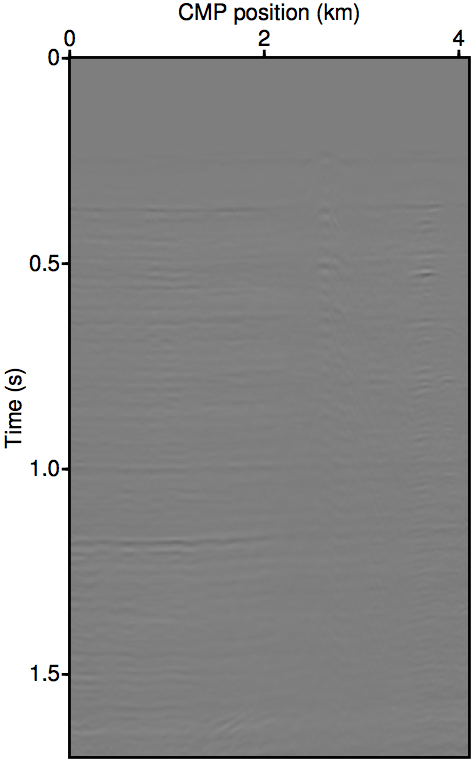
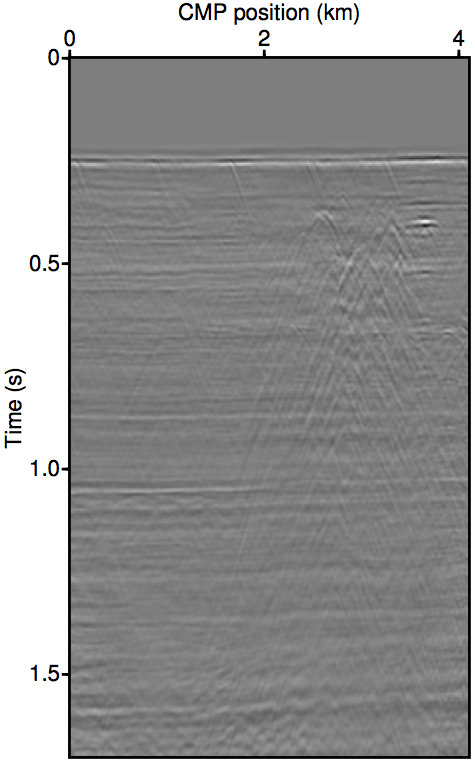
Figure 2 show the REPSI results on this field dataset with missing near-offsets using various methods. Figure 2b shows REPSI results by pre-interpolation using parabolic Radon, which is known to under-estimate near-offset amplitudes, while Figures 2c and 2d show results obtained by solving \(\widetilde{M}(\vec{G},\vec{Q};\vec{P'})\) using the re-linearization strategy. Looking at the difference plot 2f, our approach is much more successful at removing coherent multiple energy. Figure 2g shows that very little additional accuracy is gained by incorporating successively higher-order auto-convolution terms in \(\widetilde{M}(\vec{G},\vec{Q};\vec{P'})\). Finally, 2e and 2h shows a modified Gauss-Newton solution to the problem. We see relatively minor differences that is mostly phase errors.

Summary

We have presented a variation of the EPSI problem that accounts for data gaps by implicitly account for it in the inversion model without explicit data reconstruction steps. We proposed two methods to solve this new non-linear problem, and have demonstrated its efficacy on real marine streamer data. We note that this scheme does not wholly account for undersampling issues in the data, which causes more severe aliasing problems in the multiple step which cannot be wholly mitigated reliably using the approaches shown here.

Acknowledgements

We would like to acknowledge Gert-Jan van Groenestijn and Eric Verschuur for discussion with led to our involvement in EPSI. Thanks to PGS for permission to use the real dataset. This work was financially supported in part by the NSERC of Canada Discovery Grant (RGPIN 261641-06) and the CRD Grant DNOISE II (CDRP J 375142-08). This research was carried out as part of the SINBAD II project with support from the following organizations: BG Group, BGP, BP, Chevron, ConocoPhillips, CGG, ION GXT, Petrobras, PGS, Statoil, Total SA, WesternGeco, and Woodside.

References

Berkhout, A. J., & Pao, Y. H. (1982). Seismic Migration - Imaging of Acoustic Energy by Wave Field Extrapolation. Journal of Applied Mechanics, 49(3), 682. doi:10.1115/1.3162563
Fleischer, G., & Hofmann, B. (1996). On inversion rates for the autoconvolution equation. Inverse Problems, 12(4), 419–435. doi:10.1088/0266-5611/12/4/006
Fleischer, G., Gorenflo, R., & Hofmann, B. (1999). On the Autoconvolution Equation and Total Variation Constraints. ZAMM, 79(3), 149–159. doi:10.1002/(SICI)1521-4001(199903)79:3<149::AID-ZAMM149>3.0.CO;2-N
Fokkema, J. T., & Berg, P. M. van den. (1993). Seismic applications of acoustic reciprocity (p. 350). Elsevier Science. Retrieved from http://books.google.com/books?id=398SAQAAIAAJ\&pgis=1
Frijlink, M. O., Borselen, R. G. van, & Söllner, W. (2011). The free surface assumption for marine data-driven demultiple methods. Geophysical Prospecting, 59(2), 269–278. doi:10.1111/j.1365-2478.2010.00914.x
Groenestijn, G. J. A. van, & Verschuur, D. J. (2009). Estimating primaries by sparse inversion and application to near-offset data reconstruction. Geophysics, 74(3), A23–A28. doi:10.1190/1.3111115
Li, X., Aravkin, A. Y., Leeuwen, T. van, & Herrmann, F. J. (2012). Fast randomized full-waveform inversion with compressive sensing. Geophysics, 77(3), A13–A17. doi:10.1190/geo2011-0410.1
Lin, T. T. Y., & Herrmann, F. J. (2013). Robust estimation of primaries by sparse inversion via one-norm minimization. Geophysics, 78(3), R133–R150. doi:10.1190/geo2012-0097.1
Lin, T. T. Y., & Herrmann, F. J. (2014). Multilevel acceleration strategy for the robust estimation of primaries by sparse inversion. 76th eAGE conference & exhibition. Retrieved from https://www.slim.eos.ubc.ca/Publications/Public/Conferences/EAGE/2014/lin2014EAGEmas.pdf
Tibshirani, R. (1996). Regression shrinkage and selection via the lasso. Journal of the Royal Statistical Society Series B Methodological, B, 58(1), 267–288. Retrieved from http://www.jstor.org/stable/2346178
Verschuur, D. J. (1992). Adaptive surface-related multiple elimination. Geophysics, 57(9), 1166. doi:10.1190/1.1443330
Verschuur, D. J. (2006). Seismic multiple removal techniques: Past, present and future (p. 191). EAGE Publications.