Seismic Trace Interpolation with Approximate Message Passing

Navid Ghadermarzy^*, Felix J.Herrmann^*, and Özgür Yılmaz^*
*Seismic Laboratory for Imaging and Modeling (SLIM), University of British Columbia

Introduction

Regular sampling along the time axis is common approach for seismic imaging. However, seismic data are often spatially undersampled due to economical reasons as well as ground surface limitations. Too large spatial sampling interval may result in spatial aliasing. Operational conditions might also result in noisy traces or even gaps in coverage and irregular sampling which often leads to image artifacts. Seismic trace interpolation aims to interpolate missing traces in an otherwise regularly sampled seismic data to a complete regular grid.

Compressed sensing (CS) is a data acquisition technique to efficiently acquiring and recovering high-dimensional signals from seemingly incomplete linear measurements, provided that the signal is sparse or compressible in some transform domain (Candes, Romberg, & Tao, 2006; D. Donoho, 2006). Several works have shown that the structure of seismic wavefronts can be captured by a few significant transform coefficients (e.g., curvelet or Fourier coefficients) and the problem of seismic trace interpolation can be cast as a sparse recovery problem once the data is transformed into a suitable domain, e.g., discrete Fourier transform (DFT) (Liu & Sacchi, 2004; M. D. Sacchi & Ulrych, 1996), Radon transform (Hampson & others, 1986; P. Herrmann, Mojesky, Magesan, Hugonnet, & others, 2000; Thorson & Claerbout, 1985), or curvelet transform (Hennenfent & Herrmann, 2005, 2006, 2008; Naghizadeh, Sacchi, & others, 2010). Hence, the interpolation problem becomes that of finding transform domain coefficients with the smallest \(\ell_1\) norm that satisfy the subsampled measurements.

In this paper we consider two scenarios. First we consider using curvelet transform as the sparsifying transform (see, e.g., (Hennenfent & Herrmann, 2006)). Curvelet transform is a redundant transform which expands the size of the model and has been shown to be very effective in capturing the structure of the data with very few significant coefficients. Then we recover the resulting compressible signal by solving a convex minimization problem. Next we consider using Fourier transform as the transform operator. The resulting transform is not as effective as curvelet transform (in terms of sparsity of the resulting transform). However, the transformed data can still be approximated by a solving a sparse recovery problem which is much faster than the curvelet case. This is due to two reasons. First one is the availability of very fast DFT transforms and second is the applicability of approximate message passing (AMP) for this problem. AMP (D. L. Donoho, Maleki, & Montanari, 2009) is a fast (needs few matrix-vector multiplications) iterative \(\ell_1\) recovery algorithm which can be used to recover sparse Fourier coefficients (The current variants of AMP can not recover curvelet coefficients). Also notice that AMP can be used to speed up interpolation techniques that work on small high dimensional windows.\ In this paper we use AMP with Fourier transform coefficients to generate relatively good approximations of the seismic data which is used to enhance the speed and recovery performance of seismic trace interpolation in the curvelet domain. First we formulate the problem of seismic trance interpolation as a sparse recovery problem. Next we explain the approach we take to solve this problem both from the curvelet transform and Fourier transform coefficients and then we present the 2-stage algorithm which combines these two approaches.

Problem formulation

Consider a seismic line with \(N_s\) sources located on earth surface which send sound waves into the earth and \(N_r\) receivers record the reflection in \(N_t\) time samples. Rearranging the seismic line, we have a signal \(f \in \mathbb{R}^N\), where \(N=N_s N_r N_t\). Assume \(x=Sf\) where \(x\) is the sparse representation of \(f\) in some transform domain. We want to recover a very high dimensional seismic data volume \(x\) by interpolating between a smaller number of measurements \(b=RMf\), where \(RM\) is a sampling operator composed of the product of a restriction matrix \(R\), which specifies the sample locations that have data in them and a measurement basis matrix \(M\). To overcome the problem of high dimensionality, recovery is performed by first partitioning the seismic data volumes into frequency slices and then solving a sequence of individual subproblems (Mansour, Herrmann, & Yilmaz, 2013). For each partition \(j\), let \(b^{(j)}\) be the subsampled measurements of data \(f^{(j)}\) in partition \(j\) and the corresponding measurement matrix is given by \(A^{(j)}=R^{(j)}S^H\) (Notice that the superscript \(H\) denoted the Hermitian transpose and for simplicity, we have assumed the measurement matrix \(M\) to be the identity). Then for each partition we need to estimate the solution of the following minimization problem independently: \[ \begin{equation} \label{l0} \widetilde{x}^{(j)} := \underset{u}{\ \text{arg min}\ } \|u\|_0 \ \ \ \text{s.t.}\ \ A^{(j)}u=b^{(j)}, \end{equation} \] and then \(f^{(j)}\) is approximated by \(S^H \widetilde{x}^{(j)}\).

Recovery in curvelet domain with convex optimization

In this case \(S_C \in \mathbb{C}^{P \times N}\) is the curvelet transform which is used as the sparsifying transform \(S\). For each partition we use 2-D curvelet transform where \(\frac{P}{N} \approx 8\) which is highly redundant and allows for sparse representations of the data in the transformed domain. Notice that in this case \(A^{(j)}=R^{(j)}S_C^H\). The minimization problem \(\ref{l0}\) is a combinatorial problem and therefore we approximate the solution by the following convex relaxation: \[ \begin{equation} \label{l1} \widetilde{x}^{(j)}_{\ell_1} := \underset{u}{\ \text{arg min}\ } \|u\|_1 \ \ \ \text{s.t.}\ \ A^{(j)}u=b^{(j)}, \end{equation} \] and then \(f^{(j)}\) is approximated by \(S_C^H \widetilde{x}^{(j)}_{\ell_1}\). Here \(\|u\|_1=\sum\limits_{i=1}^N |u_i|\) and \(\ref{l1}\) can be efficiently solved by algorithms like SPGL1 (Van Den Berg & Friedlander, 2007).

(Mansour et al., 2013) noted that although partitioning the data using and 2-D curvelets reduces the size of the problem, it doesn’t utilize the continuity across partitions. Therefore they suggest using support set of each partition as a support estimate for the next one. For partition \(j>1\) assume \(T_j:=\text{supp}(S_CS_C^H\widetilde{x}^{(j-1)}|_k)\) which is the locations of the largest \(k\) entries of \(S_CS_C^H\widetilde{x}^{(j-1)}\) in magnitude and define the weight vector \({\rm{w}} \in \mathbb{R}^N\) such that \({\rm{w}}_j=1\) for \(j \notin T_j\) and \({\rm{w}}_j=\omega<1\) for \(j \in T_j\), where k is chosen to be the number of largest analysis coefficients that contribute 95% of the signal energy. (Mansour, Friedlander, Saab, & Yilmaz, 2012) prove that solving the following weighted \(\ell_1\) minimization results in better recovery compared to \(\ref{l1}\) if the support estimate \(T_j\) is at least 50% accurate: \[ \begin{equation} \label{weightedl1} \widetilde{x}^{(j)}_{w\ell_1} := \underset{u} {\text{argmin}} \ \| u \|_{1,{\rm{w_j}}} \ \text{s.t.} \ A^{(j)}u=b^{(j)}, \end{equation} \] where \(\|u\|_{1,{\rm{w_j}}}=\sum\limits_{i=1}^N {\rm{w}}_i|u_i|\) is the weighted \(\ell_1\) norm of \(u\).

Recovery in Fourier domain with AMP

In this case we use DFT matrix \(S_F \in \mathbb{C}^{N \times N}\) as the sparsifying operator. Hence, \(A^{(j)}=R^{(j)}S_F\) is the subsampled 2-D DFT matrix. To solve \(\ref{l0}\) the AMP algorithm (D. L. Donoho et al., 2009) starts from an initial \(x_{amp}^0\) and an initial threshold \(\hat{\tau}^0=1\) and iteratively goes by \[ \begin{equation} \label{AMP} \begin{aligned} &x_{amp}^{t+1} =\eta (x_{amp}^t+{A^{(j)}}^H z^t;\tau^t) ,\\ &z^t=y-A^{(j)} x_{amp}^t+\delta^{-1}z^{t-1}\langle \eta^{\prime} (x_{amp}^{t-1}+{A^{(j)}}^H z^{t-1};\tau^{t-1}) \rangle, \end{aligned} \end{equation} \] and \(\widetilde{x}_{amp}^{(j)}=x_{amp}^{t_{final}}\) where \(t_{final}\) is the number of times we iterate the algorithm. Here \(S_F^Hx_{amp}^t\) is the current estimate of \(f^{(j)}\), \(z^t\) is the current residual, \(\langle\cdot\rangle\) is the arithmetic mean, and \(\eta\) is the soft thresholding function \([\eta(a;s)]_j=sign(a_j)(a_j-s)_+\). This function acts on the coefficients of the signal \(a\) and zeroes out any value which is less than the scalar \(s\) in magnitude.

Similar to the previous case we can utilize the continuity of seismic data across partitions to estimate the support set of each partition. As before \(T_j:=\text{supp}(S_FS_F^Hx^{(j-1)}|_k)\) and the weight vector \({\rm{w}}\) is defined such that \({\rm{w}}_j=1\) for \(j \notin T_j\) and \({\rm{w}}_j=\omega<1\) for \(j \in T_j\). (Ghadermarzy & Yilmaz, 2013) incorporate this prior support information into the AMP algorithm by the following iterations: \[ \begin{equation} \label{weightedAMP} \begin{aligned} &x_{wamp}^{t+1}=\eta (x_{wamp}^t+{A^{(j)}}^H z^t;\tau^t {\rm{w}_j}) ,\\ &z^t=y-A^{(j)} x_{wamp}^t+\delta^{-1}z^{t-1}\langle \eta^{\prime} (x_{wamp}^{t-1}+{A^{(j)}}^H z^{t-1};\tau^{t-1} {\rm{w}_j}) \rangle, \end{aligned} \end{equation} \] The only difference between AMP and weighted AMP (WAMP) is in the value of the thresholds which is set to be a smaller value for the coefficients in the support estimate which makes them more likely to remain nonzero.

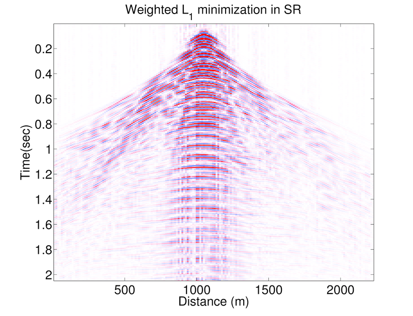
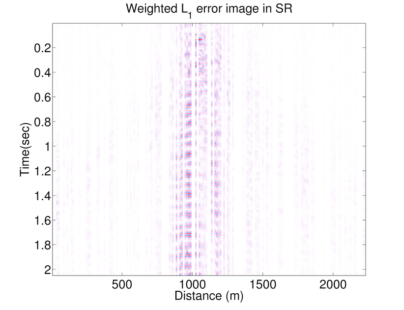
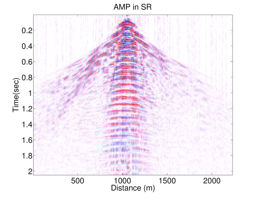
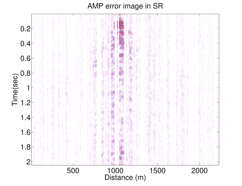
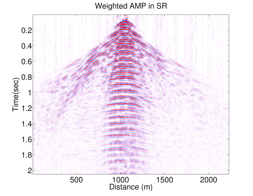
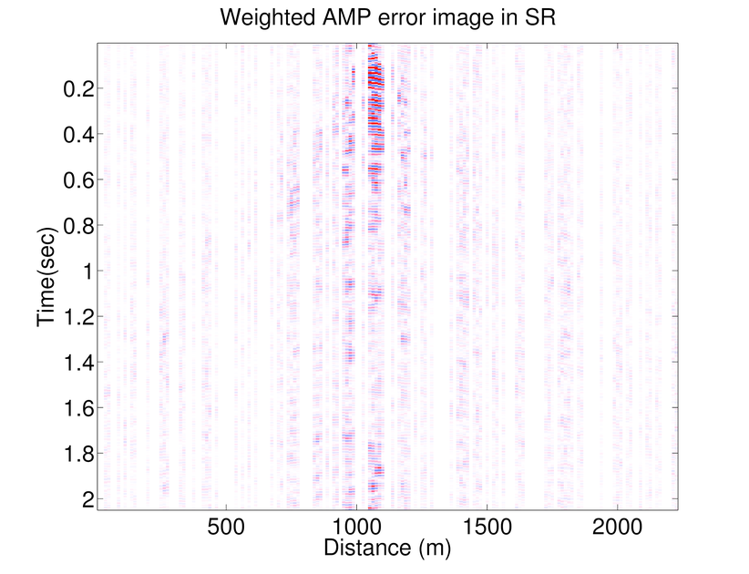
In Figure 1 .a-f we compare the performance of AMP and WAMP (in Fourier domain) with weighted \(\ell_1\) (in curvelet domain) on recovering a seismic line from the Gulf of Suez with 50% randomly subsampled receivers. The seismic line at full resolution has \(N_s = 178\) sources, \(N_r = 178\) receivers, and \(N_t = 500\) time samples acquired with a sampling interval of 4 ms. Consequently, the seismic line contains samples collected in a 1s temporal window with a maximum frequency of 125 Hz. To access the frequency slices we take the 1-D DFT of the data along time axis and interpolate the missing receivers by solving the seismic trace interpolation with weighted \(\ell_1\), AMP and weighted AMP algorithms explained above (Results of \(\ell_1\) minimization is omitted as the weighted \(\ell_1\) minimization is always giving better results (Mansour et al., 2013)). Notice that reconstruction results of weighted AMP is better than those of AMP.

2-stage algorithm

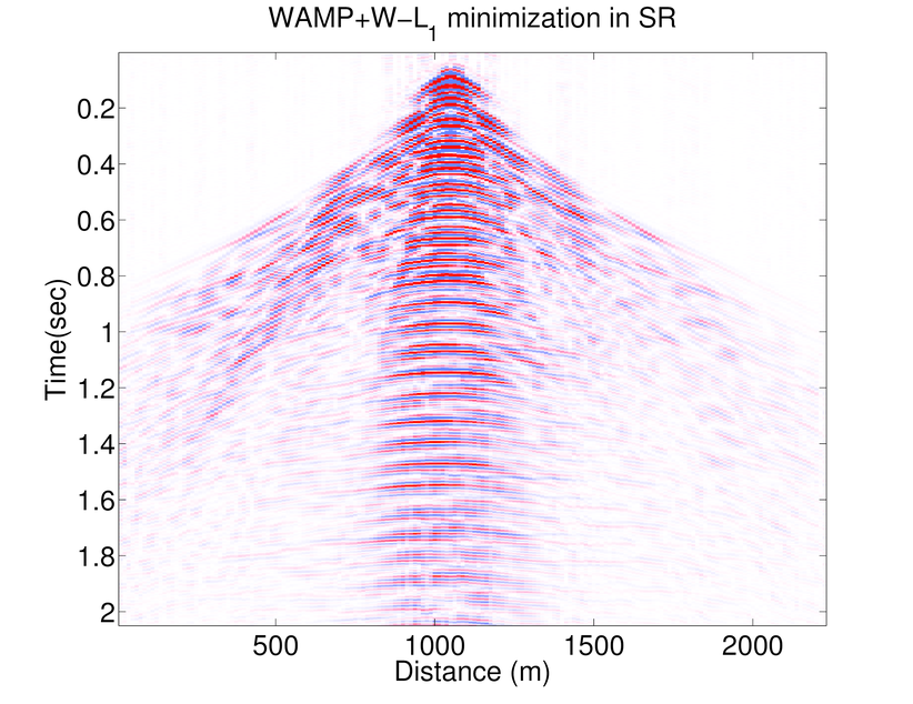
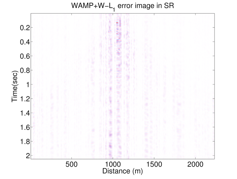
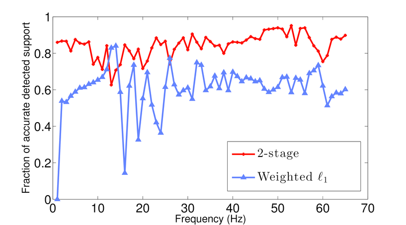
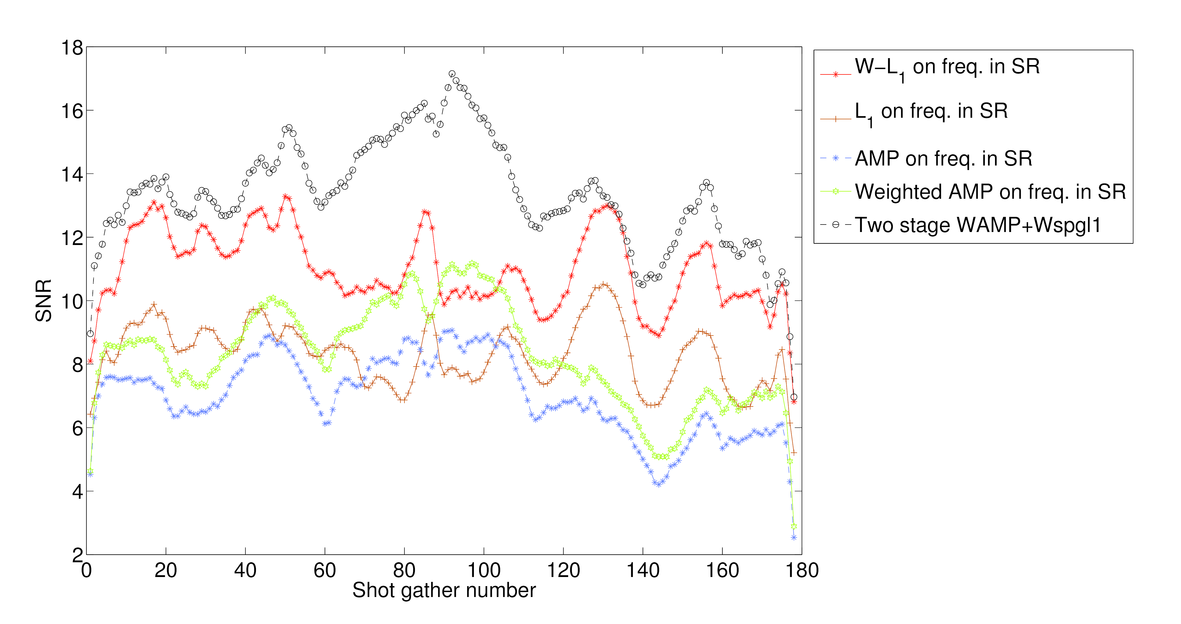
As mentioned before AMP algorithm is a significantly fast algorithm and Figure 1 shows that although the results of weighted \(\ell_1\) is better than those of weighted AMP, the results of weighted AMP is still reasonably good (considering that weighted AMP is about 40 times faster than the weighted \(\ell_1\) algorithm). Weighted \(\ell_1\) minimization in the curvelet domain gives much better results which is due to the better choice of sparsifying transform domain. On the other hand AMP is a very fast algorithm that approximates the true data reasonably good. Notice that both these algorithms are solving the same problem in different transform domains. Therefore, we can combine these algorithms to use both the fast convergence of AMP algorithm and superior results of weighted \(\ell_1\). Notice that at each partition \(j\), \(f^{(j)}\) is approximated by: \[ \begin{equation*} \begin{aligned} \text{weighted}\ \ell_1: \ \ f^{(j)} &\approx S_C^H \widetilde{x}^{(j)}_{w\ell_1} \\ \text{weighted}\ AMP: \ \ f^{(j)} &\approx S_F^H \widetilde{x}_{wamp}^{(j)} \end{aligned} \end{equation*} \] Hence the outcome of the weighted \(\ell_1\) algorithm(in the curvelet domain) can be approximated by the final outcome of the weighted AMP algorithm (which is in Fourier domain) through: \[ \begin{equation*} S_C^H\ \widetilde{x}^{(j)}_{w\ell_1} \approx S_F^H\ \widetilde{x}_{wamp}^{(j)}. \end{equation*} \] Hence, we propose a 2-stage algorithm, that for each partition \(j\) first we apply the weighted AMP algorithm \(\ref{weightedAMP}\) in the Fourier domain to get the estimate \(S_C^H \widetilde{x}^{(j)}_{w\ell_1}\). Next we use the largest coefficients of \(S_C\ S_F^H\ \widetilde{x}_{wamp}^{(j)}\) as a support estimate for \(\widetilde{x}^{(j)}_{w\ell_1}\) and solve a weighted \(\ell_1\) algorithm in the Fourier domain. Figure 2 shows an example of the accuracy achieved to predict the support of the curvelet coefficients in a seismic line when we just use the adjacent frequency slices (the weighted \(\ell_1\) case) and when we combine the information of the previous frequency slice with the approximation gained by WAMP. Here the support is chosen to be the set of largest analysis coefficients that contribute 95% of the signal energy. The estimate for the 2-stage algorithm is always better than the estimate gained by the previous slice. We also feed the approximation \(S_C\ S_F^H\ \widetilde{x}_{wamp}^{(j)}\) into the weighted \(\ell_1\) algorithm as a good initial point for the SPGL1 algorithm. As the curvelet transform is a redundant transform, we can not mathematically justify why this choice of initial point improves the convergence rate. However, empirical results show significant improvement when we feed the result of WAMP into the \(\ell_1\) algorithm. Figures 1.g and h show the recovery results by the 2-stage algorithm. In Table 1 we have compared the number of matrix-vector multiplications and average time it takes for the above algorithms to recover different frequency slices. The results of the 2-stage algorithm presented in Figure 1 uses fewer curvelet transforms compared to the weighted \(\ell_1\) which makes it faster. Figure 3 shows the SNRs achieved by \(\ell_1\), weighted \(\ell_1\), AMP, Weighted AMP, and the 2-stage algorithms for different shot gathers. The results of the 2-stage algorithm is always better than the weighted \(\ell_1\).

Recovery method	DFT transforms	Curvelet transforms	Average runtime
Weighted L1	0	1125	924s
AMP	1000	0	14s
WAMP	1000	0	14s
2-stage WAMP+WL1	1000	440	420s

Comparison of computational complexity for different recovery methods averaged over frequency slices.

Conclusions

In this abstract we showed how we can use approximate message passing for the problem of seismic trace interpolation. Due to fast nature of AMP algorithm and DFT transform we can get a good approximation of the seismic data much faster than doing the interpolation in the curvelet domain. Hence, AMP can be used as a fast preprocessor for interpolation in curvelet domain. This result shows that doing this not only improves the recovery results significantly and but also the 2-stage algorithms need less SPGL1 iterations (with curvelets) to get to a good approximation once the fast WAMP algorithms is done in the Fourier domain.

Acknowledgements

This work was financially supported in part by the Natural Sciences and Engineering Research Council of Canada Discovery Grant (RGPIN 261641-06) and the Collaborative Research and Development Grant DNOISE II (CDRP J 375142-08). This research was carried out as part of the SINBAD II project with support from the following organizations: BG Group, BGP, BP, Chevron, ConocoPhillips, CGG, ION, GXT, Petrobras, PGS, Statoil, Total SA, WesternGeco, snd woodside.

References

Candes, E. J., Romberg, J., & Tao, T. (2006). Stable signal recovery from incomplete and inaccurate measurements. Communications on Pure and Applied Mathematics, 59, 1207–1223.
Donoho, D. (2006). Compressed sensing. IEEE Transactions on Information Theory, 52(4), 1289–1306.
Donoho, D. L., Maleki, A., & Montanari, A. (2009). Message-passing algorithms for compressed sensing. Proceedings of the National Academy of Sciences, 106(45), 18914–18919.
Ghadermarzy, N., & Yilmaz, O. (2013). Weighted and reweighted approximate message passing. In SPIE optical engineering+ applications (pp. 88580C–88580C). International Society for Optics; Photonics.
Hampson, D., & others. (1986). Inverse velocity stacking for multiple elimination. In 1986 sEG annual meeting. Society of Exploration Geophysicists.
Hennenfent, G., & Herrmann, F. J. (2005). Sparseness-constrained data continuation with frames: Applications to missing traces and aliased signals in 2/3-d. In SEG international exposition and 75th annual meeting.
Hennenfent, G., & Herrmann, F. J. (2006). Seismic denoising with nonuniformly sampled curvelets. Computing in Science & Engineering, 8(3), 16–25.
Hennenfent, G., & Herrmann, F. J. (2008). Non-parametric seismic data recovery with curvelet frames. Geophysical Journal International, 173(1), 233–248.
Herrmann, P., Mojesky, T., Magesan, M., Hugonnet, P., & others. (2000). De-aliased, high-resolution radon transforms. In 70th annual international meeting (pp. 1953–1956). SEG.
Liu, B., & Sacchi, M. D. (2004). Minimum weighted norm interpolation of seismic records. Geophysics, 69(6), 1560–1568.
Mansour, H., Friedlander, M. P., Saab, R., & Yilmaz, Ö. (2012). Recovering compressively sampled signals using partial support information. IEEE Transactions on Information Theory, 58(2), 1122–1134.
Mansour, H., Herrmann, F. J., & Yilmaz, O. (2013). Improved wavefield reconstruction from randomized sampling via weighted one-norm minimization. Geophysics, 78, no. 5, V193–V206.
Naghizadeh, M., Sacchi, M., & others. (2010). Hierarchical scale curvelet interpolation of aliased seismic data. In SEG inter-national exposition and 80th annual meeting.[S. 1.]: sEG.
Sacchi, M. D., & Ulrych, T. J. (1996). Estimation of the discrete fourier transform, a linear inversion approach. Geophysics, 61(4), 1128–1136.
Thorson, J. R., & Claerbout, J. F. (1985). Velocity-stack and slant-stack stochastic inversion. Geophysics, 50(12), 2727–2741.
Van Den Berg, E., & Friedlander, M. (2007). SPGL1: A solver for large-scale sparse reconstruction. Online: http://www. Cs. Ubc. Ca/Labs/Scl/Spgl1.