Extending the search space of time-domain adjoint-state FWI with randomized implicit time shifts

Mathias Louboutin^* and Felix J. Herrmann
Seismic Laboratory for Imaging and Modeling (SLIM), The University of British Columbia

Introduction

To reduce the dependence of full-waveform inversion (FWI, (Virieux and Operto, 2009)) on the quality of starting models, we apply recent work by Burke et al. (2005) on non-convex/non-smooth optimization to adjoint-state FWI in the time-domain. By using this technique, we intend to tackle an important limitation of classical adjoint-state methods that ask for a starting that too accurate to be practical. Our approach is similar in spirit to other methods aimed to overcome cycle skip problems but instead of extending the search space—as for instance in Wavefield Reconstruction Inversion (WRI, Leeuwen et al. (2014), Leeuwen and Herrmann (2015)) where both the velocity model and wavefields are unknowns—our method extends the search space implicitly while relying on robust gradient sampling algorithm for nonsmooth, nonconvex optimization problems (Burke et al., 2005). By working on sets of nearby velocity models instead of working with a single velocity model as in conventional adjoint-state, our approach scales to high frequencies in 3D at low computational and memory overhead. To set the stage, we start by introducing the gradient sampling algorithm followed by our proposal how to incorporate this technique into FWI without incurring massive computational costs. We conclude by demonstrating the advantages of this method compared to regular FWI on a synthetic but realistic 2D model.

Gradient sampling for FWI

While smooth, i.e. the objective of FWI is differentiable with respect to the velocity model, FWI is non-convex and suffers as a consequence from local minima and sensitivity to starting models. A recent result by Curtis and Que (2013) extends Burke et al. (2005)’s original work on gradient sampling for non-smooth optimization problems to non-convex problems with encouraging results. Encouraged by these findings we propose to adapt this method to overcome issues related to the non-convexity of FWI. As a result, we expect the proposed method to make FWI less reliant on accurate starting models. As we show below, the cornerstone of this algorithm is to work with local neighborhoods (read sets of perturbed velocity model around the current model estimate) instead with a single velocity model. By working with these neighborhoods, we are able to reap global information on the objective from local gradient information at small cost.

Gradient sampling for non-smooth and non-convex optimization

We minimize at iteration \(k\) the objective function \(\Phi(\vd{x})\) with respect to the unknown variable \(\vd{x} \in \!R^N\) by using local gradient \(\nabla\Phi(\vd{x})\) information by

• sampling \(N+1\) vectors \(\vd{x}_{ki}\) in a ball \(B_{\epsilon_k}(\vd{x}_k)\) defined as all \(\vd{x}_{ki}\) such that \(\norm{\vd{x}_k-\vd{x}_{ki}} < \epsilon_k\), where \(\epsilon_k\) is the maximum distance between the current estimate and a sampled vector;
• calculating gradients for each sample—i.e., \(\vd{g}_{ki} = \nabla\Phi(\vd{x}_{ki})\);
• computing descent directions as a weighted sum over all sampled gradients—i.e., \[ \begin{equation} \vd{g}_k \simeq \sum_{i=0}^p \omega_i\vd{g}_{ki} \text{ , such that }\sum_{i=0}^p \omega_i = 1,\ \omega_i>0 \ \forall i \label{GSdir} \end{equation} \]
• updating the model according to \(\vd{x}_{k+1} = \vd{x}_{k} - \alpha \vd{H}^{-1} \vd{g}_k\), where \(\alpha\) is a step length obtained from a line search and \(\vd{H}^{-1}\) is an approximation of the inverse Hessian.

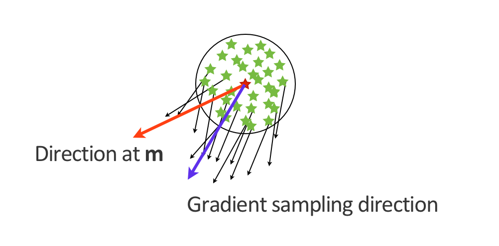
We illustrate the calculation of a single iteration of this algorithm in Figure 1. While the above procedure demonstrably is capable of finding minima of non-convex minimization problems using local gradient information only, its computational costs are prohibitive. For instance, for a model of size \(N\) (in number of grid points) we would need to calculate \(N+1\) gradients, a cost way out of reach for even the smallest FWI problem. The other major drawback is that the obtention of the weights \(\omega_i\)requires the solution of a quadratic subproblem over all the gradients \(\vd{g}_{ki}\), which requires too much storage. We circumvolve these issues in two ways. First, we approximate the solution of the quadratic subproblems with predetermined random positive weights. This choice will not always give accurate gradient sampling weights but will always guaranty that the obtained update direction will perform as well as FWI in the worst case and as well as gradient sampling in the best case. Random weights that satisfy the constraints (positive and sum to one) of the subproblem improve then the chances to be in the best case scenario as the descent direction will be a non-optimal but feasible solution of the subproblem. Secondly, we exploit the structure of time-stepping solutions of the wave equation to build an implicit approximation of sampling of velocity models in the ball \(B_{\epsilon_k}(\vd{x}_k)\)

Implicit time shift and on-the-fly Gradient sampling

As we just stated, gradient sampling relies on the computation of gradients at (too) many sampling points in the neighborhood of the current model. Unfortunately, this requirement is not feasible in a realistic setting because gradients of the FWI objective \(\Phi_s(\vd{m})\) for an acoustic medium (Virieux and Operto, 2009) involves \[ \begin{equation} \nabla\Phi_s(\vd{m})=-\sum_{\vd{t} \in I} \left[ \text{diag}(\vd{u}[\vd{t}]) (\vd{D}^\top \vd{v} [\vd{t}]) \right], \label{GradientAdj} \end{equation} \] where \(\vd{m}\) is the square slowness and \(\vd{q}_s\) the source. In this expression, the superscript \(\top\) denotes the transpose and the matrix \(\vd{D}\) contains the upwind discretization of the second-order time derivative \(\frac{\delta^2}{dt^2}\). The sum in this expression for the correlation between the forward \(\vd{u}\) and adjoint \(\vd{v}\) wavefields, calculated from \[ \begin{equation} {A}(\vd{m})\vd{u} = \vd{q}_s, \ \ \ {A}^\top(\vd{m}) \vd{v} = \vd{P}_r^\top \delta\vd{d}_s, \label{Fw} \end{equation} \] runs over the time index set \(I\) and involves inverting the discrete acoustic wave equation operator \({A}(\vd{m})\), the receiver projection operator \(\vd{P}_r\) and the data residual \(\delta\vd{d}_s\). As we can see, these gradient calculations require the solution of at least two PDEs so generating \(N\) gradient would require at least \(2N\) PDE solves. However, as we will show below we can reduce these costs to only two PDE solves by randomly perturbing the velocity at each time step. Our main argument is based on the fact that the effects of slightly perturbed velocity models contained within the vicinity of the current velocity model can be approximated by time shifts. This means that we can obtain approximations of of the forward and reverse-time wavefields corresponding to perturbed velocity models, in the neighborhood of our current model estimate, by simply time shifting these wavefields. So, we argue that for a slightly perturbed velocity model \(\tilde{\vd{m}}\) nearby \(\vd{m}\), we can write \[ \begin{equation} \vd{u(\tilde{\vd{m}})}[\vd{t}] \approx\vd{u(m)}[\vd{t}+\tau], \ \ \ \vd{v(\tilde{\vd{m}})}[\vd{t}] \approx\vd{v(m)}[\vd{t}-\tau]. \label{TSWF2} \end{equation} \] Note that the shift in time \(\tau\) is reversed for the adjoint wavefield as the propagation time axis is reversed (propagated backward in time). With this approximation, we can now write a simplified expression for the corresponding gradients with respect to perturbed models \(\tilde{\vd{m}}\) : \[ \begin{equation} \nabla\Phi_s(\tilde{\vd{m}})=-\sum_{\vd{t} \in I} \left[ \text{diag}(\vd{u}[\vd{t}+\tau]) (\vd{D}^\top \vd{v} [\vd{t}-\tau]) \right]. \label{GsGrad} \end{equation} \] We now have a way to compute multiple gradients for a range of velocity models in the neighborhood \(B_{\epsilon_k}(\vd{x}_k)\) at roughly the same computational cost incurred when calculating the usual FWI gradient. Moreover, by limiting the maximum time shift to \(\tau_{max}=\frac{1}{f_0}\), where \(f_0\) is the peak frequency of the source wavelet, we effectively define neighborhoods \(B_{\epsilon_k}(\vd{x}_k)\) at each iteration \(k\). With this choice, we guaranty wavefields not to be shifted by more than half a wavelength meaning we only consider shifts contained within a single wavefront. While the above described method allows us to apply time shifts as proxies for evaluating gradients in perturbed velocity models, it requires storage of the forward and reverse-time (adjoint) wavefield — an unfeasible proposition. To overcome this memory issue, we propose to use recently developed technique that allows us to work with drastically (10\(\times\)) randomly time subsampled wavefields (Louboutin and Herrmann, 2015). We mitigate artifacts induced by this time subsampling by generating different jitter sampling sequences for each shot such that maximum time gaps are controlled and coherent artifacts are prevented from building up. To avoid storage and explicit calculations of gradients for each perturbed model, we approximate the descent directions implicitly by weighted sums evaluated at jittered time samples:

\[ \begin{equation} \begin{split} \overline{\nabla\Phi_s(\vd{m})}:= -\sum_{t \in \bar{I}} \left[ \text{diag}(\bar{\vd{u}}[\vd{t}]) (\overline{\vd{D}^\top \vd{v}}[\vd{t}]) \right], \ \ \ \bar{\vd{u}} = \sum_{\vd{t}=t_i}^{t_{i+1}} \alpha_t \vd{u}[\vd{t}], \ \ \ \overline{\vd{D}^\top \vd{v}} = \sum_{\vd{t}=t_i}^{t_{i+1}} \alpha_t \vd{D}^\top \vd{v}[\vd{t}]. \\ \end{split} \label{GSGradTC} \end{equation} \]

where \(\bar{I}=[t_1, t_2, ..., t_n]\) are the jittered time sampled from \([1,2,3,...,n_t]\). We arrived as these expressions, where \(\alpha_t>0\)’s are random weights chosen such that \(\sum{\alpha_t} = 1\), by expanding and factorizing the sum as a function of common time-shifts. We avoid the need of extra storage because we calculate these averaged wavefields on the fly and store them during forward propagation. The averaged adjoint wavefield is computed during back propagation. Details of our implicit gradient sampling scheme are included in Algorithm 1, where \(H^{-1}\) is the inverse of quasi-Newton Hessian.

Input: Measured data \(\vd{d}\) and starting model \(\vd{m}_0\)
Result: Estimate of the square slowness \(\vd{m}_{k+1}\) via Gradient Sampling adjoint state
1. Set the subsampling ratio for the wavefield \(\tau_{max}\)
2. For k=1:niter
    3. For s=1:nsrc
       4. Draw an new set of time indices \(\bar{I}\) for the wavefields for each shot
       5. Compute the average forward wavefield \(\bar{\vd{u}}\) via Equation \(\ref{Fw}\) & [#ubar] (on the fly sum)
       6. Compute the gradient via Equation \(\ref{GSGradTC}\) (on the fly sum of the adjoint)
       7. Stack with the previous gradients \(\vd{g}=\vd{g}+\overline{\nabla\Phi_s(\vd{m}_k)}\)
    8. End
    9. Get the step length \(\alpha\) via linesearch 
   10. Update the model \(\vd{m}_{k+1}=\vd{m}_{k}-\alpha\vd{H}^{-1}\vd{g}\)

Example

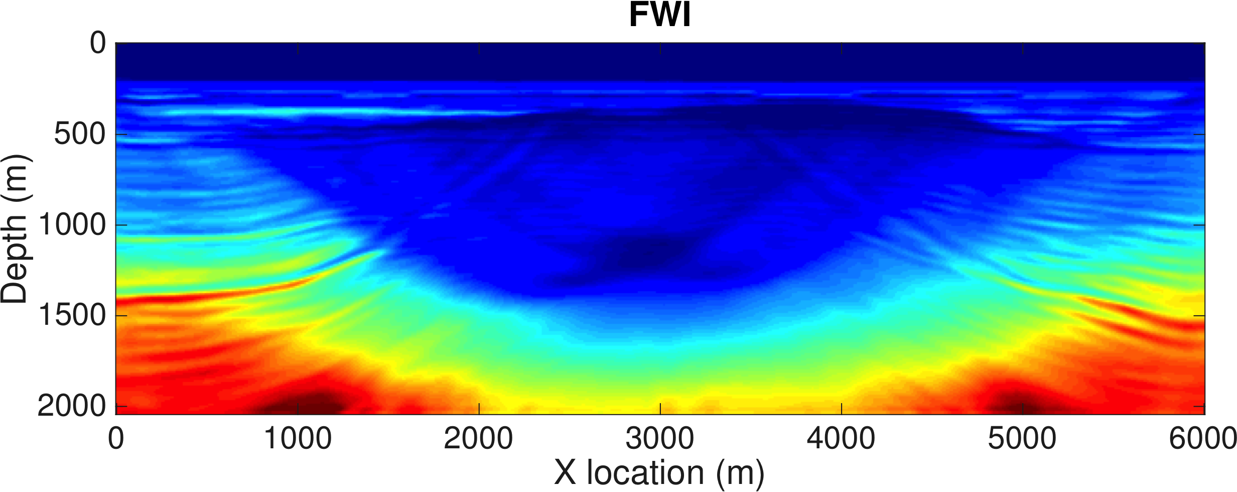
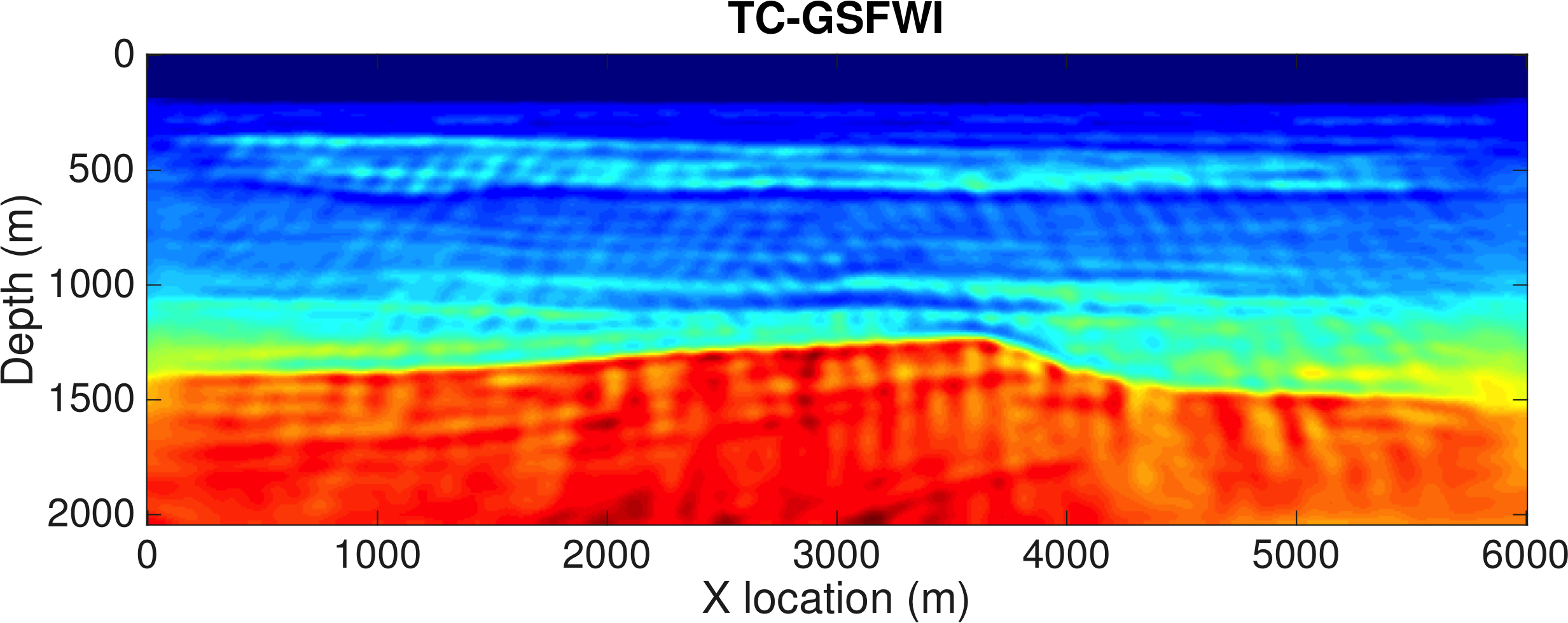
We demonstrate our method on a synthetic 2D model and include results from conventional FWI for comparison. To illustrate the advantage of our Time-Compressed Gradient Sampling FWI algorithm (TC-GSFWI), we deliberately choose a poor starting model, yielding a conventional FWI result that is cycle skipped (See Figure ), derived from the synthetic BG’s Compass model. Aside from being complex, i.e., the model contains fine-scale heterogeneity constrained by well data, this model has a challenging velocity kick back at 800 m depth that is not present in the starting model. In our experiment, we use 50 sources located at \(100\mathrm{m}\) intervals and at \(25\mathrm{m}\) depth, 201 receivers at \(25\mathrm{m}\) intervals at \(100\mathrm{m}\) depth (at the ocean bottom) and a Ricker wavelet with a \(15\mathrm{Hz}\) peak frequency as a source. The total recording time is \(4\mathrm{s}\) and the shot records are sampled at \(4\mathrm{ms}\). As described above, the subsampling ratio for our TC-GSFWI algorithm is set according to the peak frequency of the wavelet, yielding jittered subsampled wavefields at an average temporal sampling interval of only \(100\mathrm{ms}\). Because the randomized jittering samples on average at 25 % of Nyquist, we achieve a reduction in memory cost of 95% compared to memory requirements of conventional FWI. The inversion itself is carried out with a projected quasi-Newton method The inverted velocity models are shown in Figure 2. We observe that the initial velocity model is indeed cycle skipped for FWI, as the result shows a global low velocity instead of the layered shape structure of the true model. The inverted velocity with GSFWI, on the other hand, includes the main features of the true velocity model. This result is consistent with the fact that gradient sampling uses global information to minimize non-convex objectives—i.e., objectives with local minima due to cycle skipping. While our method for this example is clearly less sensitive to the quality of the starting model, the jitter sampling and implicit velocity perturbations lead to inversion artifacts. These artifacts can be removed by either composing certain (smoothness) constraints on the model or by reusing this inversion as a starting model for conventional FWI with these constraints. This inversion result is exciting because it reduces memory usage and was obtained at approximately the same computational cost as conventional FWI.

Conclusions

By combining randomized time subsampling in conjunction with the observation that random time shits applied to the forward and reverse-time wavefields can be considered as proxies for wavefields generated in randomly perturbed velocity models, we arrive at a computationally feasible formulation of gradient sampling for full-waveform inversion. Compared to ordinary gradient based algorithms, gradient sampling reaps global information making it suitable to minimize non-convex optimization problems. While we do not have a formal proof of our method, there are indication that our method is less sensitive to cycle skips. As a byproduct of the randomized sampling, we are also able to significantly reduce the storage requirements of gradient calculations making our method suitable for 3D models.

Acknowledgements

This research was carried out as part of the SINBAD II project with the support of the member organizations of the SINBAD Consortium.