Data normalization strategies for full-waveform inversion

Introduction

Full Waveform Inversion (FWI) is a seismic inverse problem that aims to match observed data and numerically simulated synthetic data sample by sample to produce high-quality, high-resolution velocity models of the subsurface. The sample-wise nature of the matching operation between the two datasets requires that a reasonable amplitude coherency between the two datasets exist. Amplitude corrections range from a single scalar to an array with the same size as the data. The former, single scalar represents a general scaling factor that can be applied to the observed data as a pre-processing step. On the other end of the spectrum, we have strategies aimed at matching relative amplitudes (Rajagopalan, 1987), which compensate for the inaccurate physics in the numerical approximation of the wave equation; these time-varying schemes are difficult to differentiate to obtain suitable expressions for their objective function gradients. We propose two intermediate schemes: shot-by-shot and trace-by-trace normalization. In the presented examples we assume that both amplitude and phase spectral shapes are known but their absolute sizes are not and we explore the effects of correcting these various scaling mismatches in the objective function definition and in the adjoint source.

Formulations

We describe strategies that are applied to synthetic and observed data, restricting our analysis to methods that apply the same normalization method to both datasets. Because the normalization schemes we introduce are data dependent, we differ from normalization techniques that apply the same normalization factor to both dataset and keep the gradients and adjoint sources expressions unchanged. We derive here analytical expressions for the objective functions, adjoint sources and gradients non-linear normalization schemes. We restrict ourselves to the \(\ell^2\) norm, but extensions to other norms is currently investigated.

Non-normalized FWI

Consider the usual adjoint-state FWI formulation (Virieux and Operto, 2009,Haber et al. (2012)): \[ \begin{equation} \begin{aligned} \minim_{\vd{m}} \Phi(\vd{m})&=\frac{1}{2}\norm{\vd{d}_s - \vd{d}_0}^2 \\ \vd{d}_s &= \vd{P}_r\vd{A}(\vd{m})^{-1}\vd{q} \end{aligned} \label{AS} \end{equation} \] where \(\vd{m}\) is the squared slowness, \(\vd{u}\) is the forward wavefield, \({A}(\vd{m})\) is the discretized wave equation, \(\vd{q}\) is the source and \(\vd{d}\) is the observed data. The main pitfall of this formulation is amplitude fitting. The amplitude of the synthetic wavefield \(\vd{u}\) depends on the space and time discretization and the magnitude of \(\vd{q}\). Considering the unknown velocity, density, …, it is very unlikely to simulate a wavefield with amplitudes matching the observed data. Amplitude fitting is then necessary and, with non-linear normalization, requires an adequate rewrite of the objective function. We introduce two normalized optimization problems that accept any solution aligned with the observed data (of the form \(\vd{d}_s = \alpha \vd{d}_0\) for any \(\alpha > 0\)) as a minimizer, or from a data side, tries to find a model that generates data only differing by a constant from the true data.

Normalized objective

At first, we look at a normalized objective function. The normalization is done on the objective function side and normalizes both datasets by their respective norms. \[ \begin{equation} \minim_{\vd{m}} \Phi(\vd{m}) = \frac{1}{2}\norm{\frac{\vd{d}_s}{\norm{\vd{d}_s}} - \frac{\vd{d}_0}{\norm{\vd{d}_0}}}^2. \label{Norm_obj} \end{equation} \] The normalization is non-linear (depends on the synthetic data and therefore on the velocity) in this case and the gradient with respect to the square slowness \(\vd{m}\) has to be derived taking the normalization into account. Following differential calculus basic rules results in the following expression for the gradient (where the synthetic data is denoted by \(\vd{d}_s\) to simplify the expression): \[ \begin{equation} \begin{aligned} \nabla_m\Phi(\vd{m})&= \vd{J}^T \vd{r} = -(\frac{\vd{d}^2\vd{u}}{\vd{d} \vd{t}^2})^T\vd{A}(\vd{m})^{-T}\vd{P}_r^T \vd{r}.\\ \vd{r} &= \frac{1}{\norm{\vd{d}_s}}(\frac{\vd{d}_s}{\norm{\vd{d}_s}} \frac{\vd{d}_s^T \vd{d}_0}{\norm{\vd{d}_s}\norm{\vd{d}_0}}- \frac{\vd{d}_0}{\norm{\vd{d}_0}}) \end{aligned} \label{Grad_Norm_obj} \end{equation} \] where \(\vd{J}\) is the Jacobian operator of the usual non-normalized adjoin-state formulation. The term \(\vd{d}_s^T \vd{d}_0\) in this expression is correcting for the phase mismatch between the observed and synthetic data in the adjoint source.

Normalized adjoint source

For the second method, we choose the adjoint source to be a normalized data residual and derive the corresponding objective function from it. The adjoint source is chosen to be \[ \begin{equation} r =\frac{\vd{d}_s}{\norm{\vd{d}_s}} - \frac{\vd{d}_0}{\norm{\vd{d}_0}}. \label{Norm_adj} \end{equation} \] and the FWI gradient is then \[ \begin{equation} \nabla_m\Phi(\vd{m})= \vd{J}^T \vd{r}. \label{Grad_Norm_adj} \end{equation} \] Knowing \(\vd{J}^T\frac{\vd{P}_r\vd{A}(\vd{m})^{-1}\vd{q}}{\norm{\vd{P}_r\vd{A}(\vd{m})^{-1}\vd{q}}} = \frac{d\norm{\vd{P}_r\vd{A}(\vd{m})^{-1}\vd{q}_s}}{d\vd{m}}\), we obtain the corresponding objective function: \[ \begin{equation} \minim_{\vd{m}} \Phi(\vd{m}) =\norm{\vd{P}_r\vd{A}(\vd{m})^{-1}\vd{q}} - \frac{(\vd{P}_r\vd{A}(\vd{m})^{-1}\vd{q})^T \vd{d}_0}{\norm{\vd{d}_0}} \label{Norm_adj_obj} \end{equation} \] This objective function is not quadratic with respect to the residuals anymore but compares how aligned with \(\vd{d}_0\) the synthetic data is. The objective function in this case can also be rewritten as \[ \begin{equation} \minim_{\vd{m}} \Phi(\vd{m}) = (\vd{P}_r\vd{A}(\vd{m})^{-1}\vd{q})^T \left(\frac{\vd{P}_r\vd{A}(\vd{m})^{-1}\vd{q}}{\norm{\vd{P}_r\vd{A}(\vd{m})^{-1}\vd{q}}} - \frac{\vd{d}_0}{\norm{\vd{d}_0}} \right). \label{Norm_adj_obj2} \end{equation} \] Similarly to conventional FWI, the difference between the synthetic and observed data is still taken into account. Moreover, the objective function also considers how much the observe correlates with the synthetic data. The gradient on the other hand is a straightforward FWI gradient with a normalized adjoint source (the forward wavefield is unchanged), but the correct objective function formula is required for any optimization algorithm assessing minimum decrease of the objective to update the model.

Shot-by-shot vs trace-by-trace

Shot-by-shot or trace-by-trace strategies will have different consequences. On one hand, normalizing on a shot-by-shot basis acts as a very crude form of source estimation in the sense that we are after a scalar that matches the energy of both \(\vd{d}_s\) and \(\vd{d}_0\) for the whole shot gather. This strategy conserves the natural amplitude decay with offset. Normalization trace-by-trace, on the other hand, has a strong influence on the energy balance in the gradients since traces at larger offsets contribute as much to the gradient formation as those at close offsets. This results in a better balanced illumination coverage (as offset from the source increase), but has the disadvantage that traces that are more likely to be cycle-skipped (long offset) have the same weight as traces that are at short offsets, increasing the risk of falling in a local minimum if the starting model is not good enough.

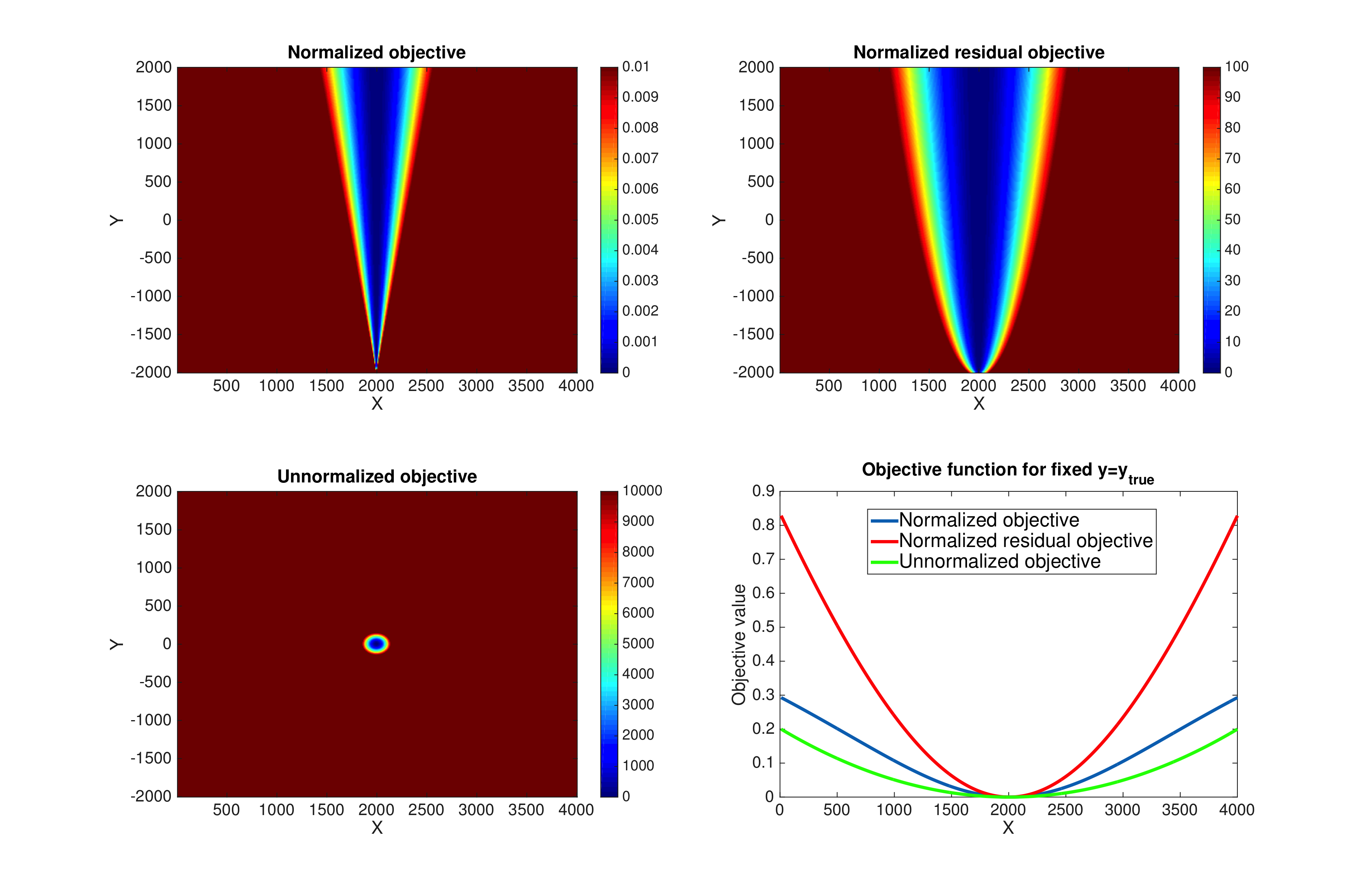
Objective function shapes

We show the shape of the objective functions in a simple two dimensional case for the non-normalized, normalized objective and normalized adjoint source cases on Figure 1. The equivalent geophysical setup would be a single trace experiment with two time samples. The displayed images represent the objective functions values for a range of traces around the true solution. We observe that FWI only accepts the true solution as the minimizer while both normalized formulations accept any solution aligned (\(\vd{d}_0 = \alpha \vd{d}_s\), \(\alpha > 0\)) with the true solution as a minimizer removing any amplitude uncertainty. The slice of the objective functions shows that the objective function associated with a normalized adjoint source is much narrower/steeper allowing better progress toward the solution.

Example

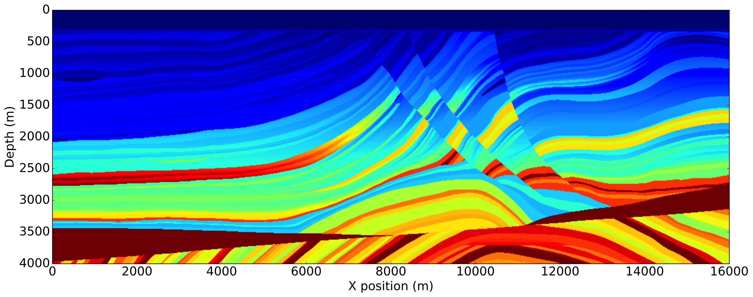
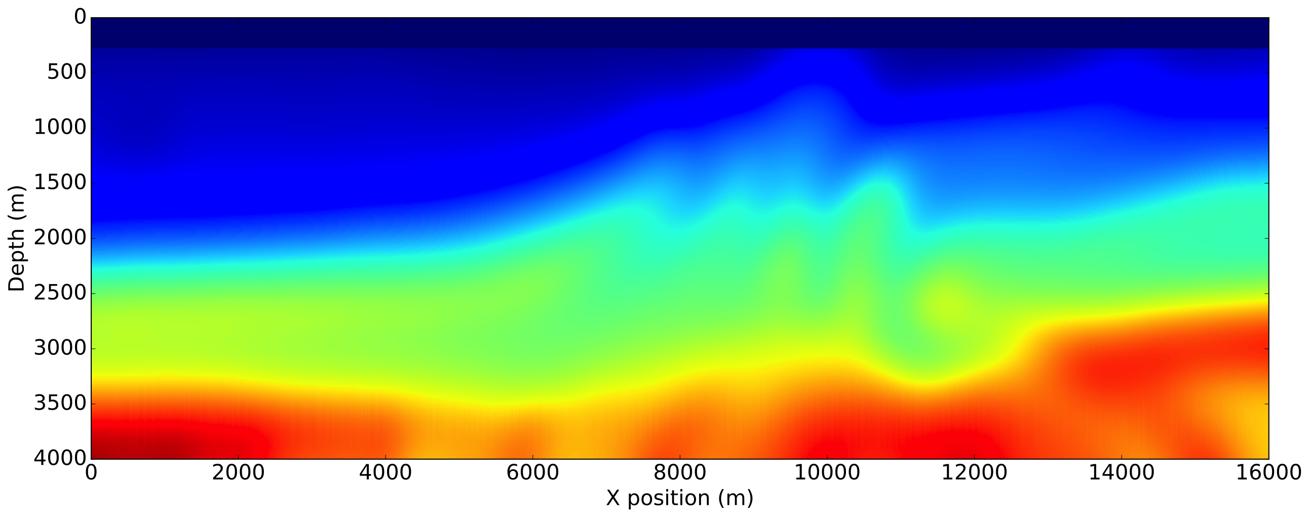
We illustrate the impact of our normalization methods on the Marmousi-ii model (Versteeg, 1994). The model size is \(4\mathrm{km}\)x\(16\mathrm{km}\) discretized with a \(10\mathrm{m}\) grid in both directions. We use a \(8\mathrm{Hz}\) Ricker wavelet with \(5\mathrm{s}\) recording. The receivers are placed at the ocean bottom every \(12.5\mathrm{m}\). The initial velocity model is a smoothened version of the true velocity model by a Gaussian filter and is accurate enough to consider the non-normalized FWI gradient computed with the true source as a reference. We show the true model, initial model and true perturbation on Figure 2.

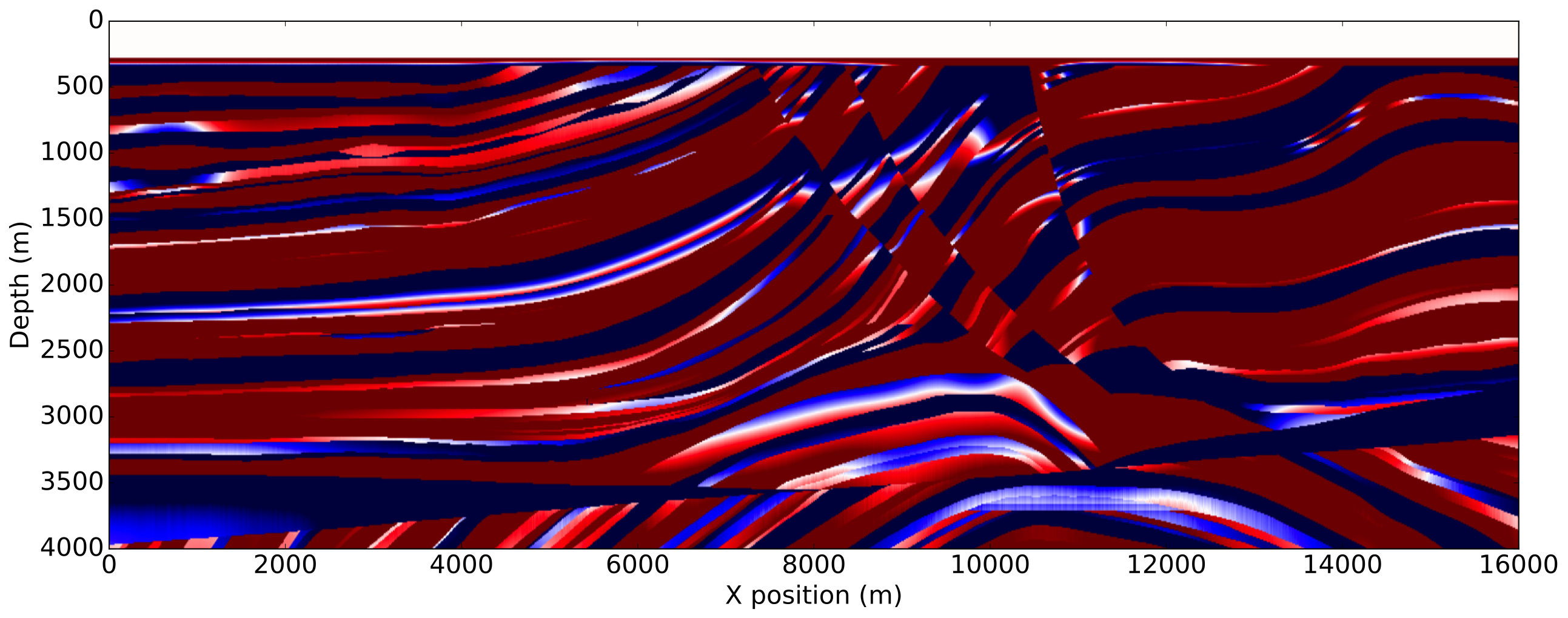
To enforce amplitude error in the data fit, we use a wrongly scaled version of the true source for inversion. The FWI gradient obtained with the true source, corresponding to the most ideal case, is then used as reference. The gradients obtained with the proposed methods are shown on Figure 3.

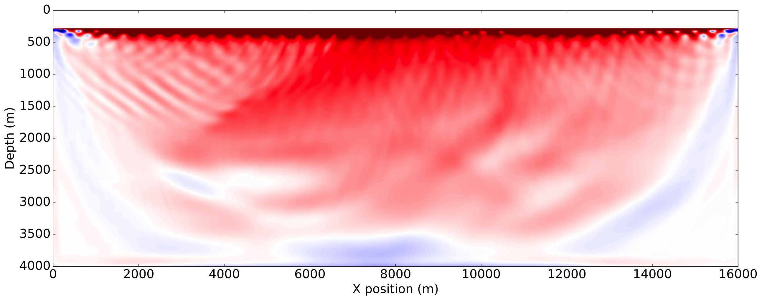
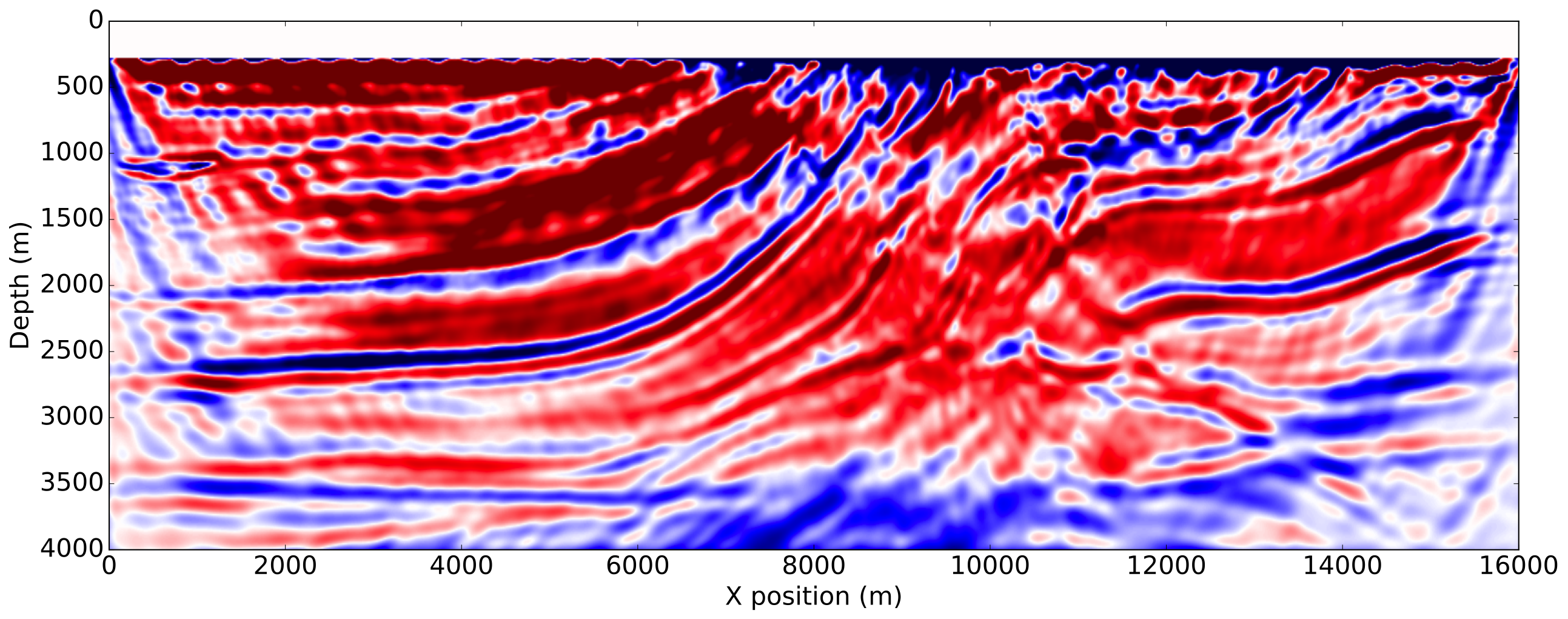
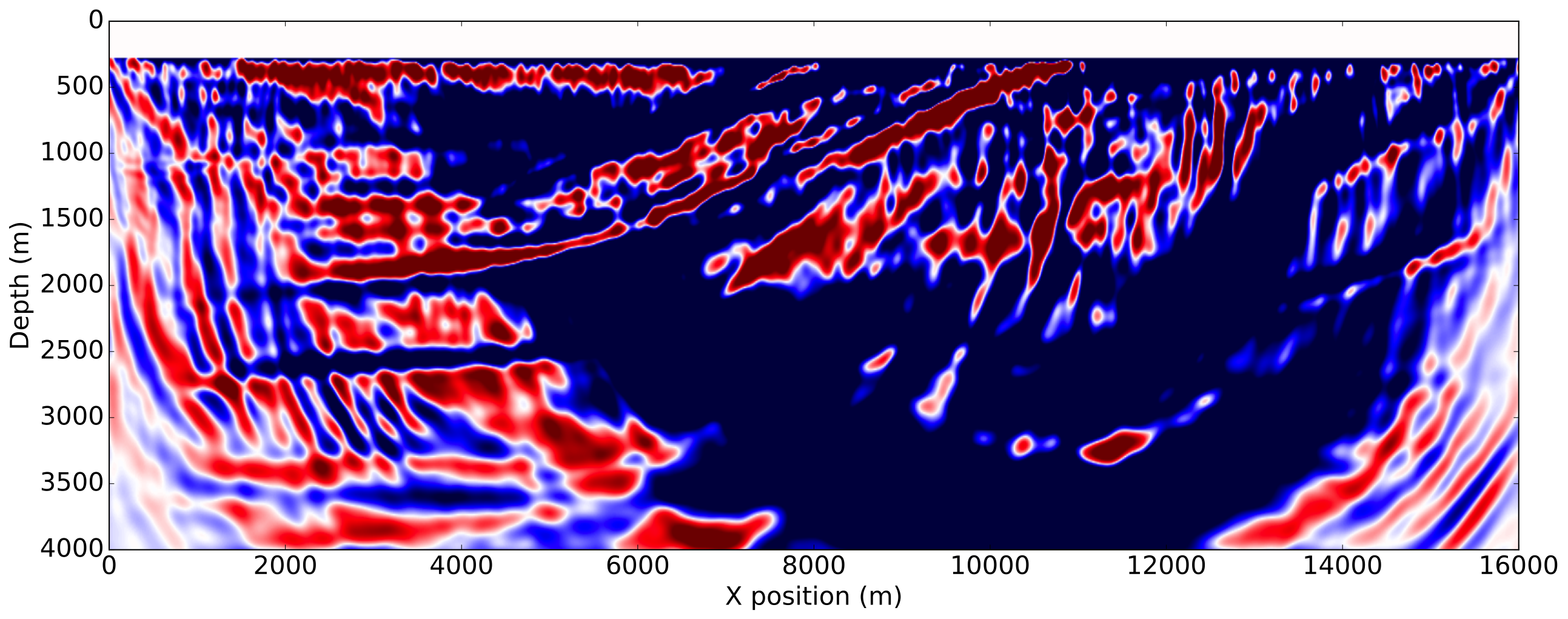
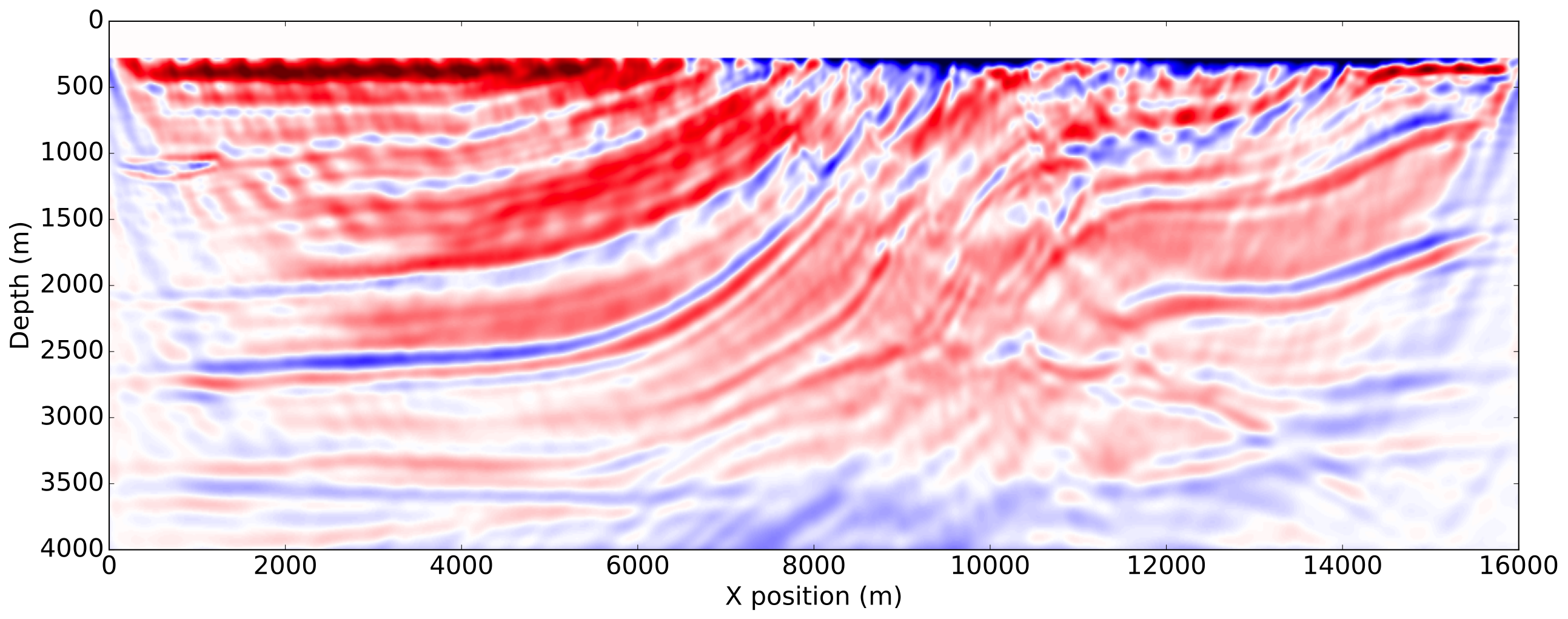
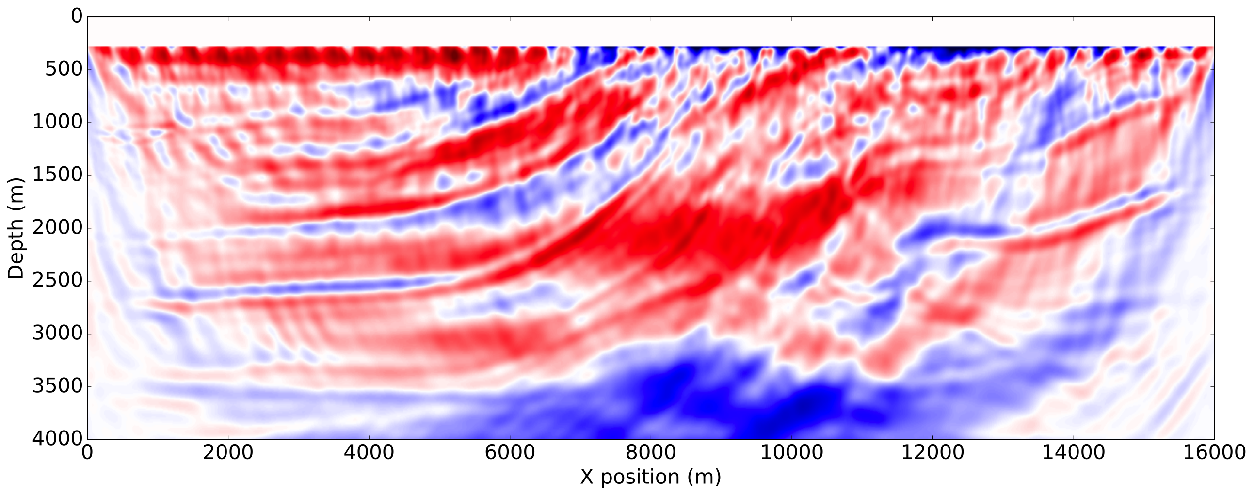
As expected from a good initial model, the FWI gradient with the true source shows most of the features present in true perturbation and is a good update direction for inversion. The gradient obtained with both normalization methods using a shot-by-shot strategy is very similar to the true source gradient and the true perturbation as well demonstrating the amplitude free property of our methods. On the other hand, we see that a trace-by-trace normalization strategy with a normalized objective generates a cycle skipped gradient and will not update the model properly. This is a consequence of the phase correction on the adjoint source at large offsets and highlights the risks of a trace-by-trace strategy discussed earlier. Finally, we see that a trace-by-trace strategy or the normalized adjoint source formulation still provides a good update direction, even though the gradient contains less details than the shot-by-shot results but has a better illumination balance between the shallow and the deeper part of the model.

Conclusion

We showed that data normalization provides an automatic way to mitigate amplitude uncertainties and improves the inversion results compared to a naive FWI implementation when there are errors in the absolute source magnitude. Our results suggest that trace normalization is less reliable than shot normalization even though a normalized adjoint source formulation is more robust to large offset mismatches. Secondly, we showed that shot-by-shot normalization strategies are well suited for amplitude mismatch correction in seismic inversion. Considering that a complete algorithm for FWI uses iteratively gradient information, the behaviour observed in a single gradient should extend to the inversion result. Even though this methods require a known source time signature, one could combine it with a source estimation method and guarantee that any amplitude ambiguity in the source estimation would be cancelled out.

Acknowledgements

This research was carried out as part of the SINBAD II project with the support of the member organizations of the SINBAD Consortium.