A lifted \(\ell_1/\ell_2\) constraint for sparse blind deconvolution

Abstract

We propose a modification to a sparsity constraint based on the ratio of \(\ell_1\) and \(\ell_2\) norms for solving blind seismic deconvolution problems in which the data consist of linear convolutions of different sparse reflectivities with the same source wavelet. We also extend the approach to the Estimation of Primaries by Sparse Inversion (EPSI) model, which includes surface related multiples. Minimizing the ratio of \(\ell_1\) and \(\ell_2\) norms has been previously shown to promote sparsity in a variety of applications including blind deconvolution. Most existing implementations are heuristic or require smoothing the \(\ell_1/\ell_2\) penalty. Lifted versions of \(\ell_1/\ell_2\) constraints have also been proposed but are challenging to implement. Inspired by the lifting approach, we propose to split the sparse signals into positive and negative components and apply an \(\ell_1/\ell_2\) constraint to the difference, thereby obtaining a constraint that is easy to implement without smoothing the \(\ell_1\) or \(\ell_2\) norms. We show that a method of multipliers implementation of the resulting model can recover source wavelets that are not necessarily minimum phase and approximately reconstruct the sparse reflectivities. Numerical experiments demonstrate robustness to the initialization as well as to noise in the data.

Introduction

The problem of recovering a source wavelet \(w\) and sparse reflectivity signals \(x_j\) from redundant traces \(f_j\) can be modeled as a blind deconvolution problem. We assume \(w\) is the same for each included trace and consider two convolution models. The simplest model, as described for example in (Ulrych and Sacchi, 2006), is given by \[ \begin{equation} \label{BD} f_j = x_j \ast w \ , \ \ j = 1,...,n\ , \end{equation} \] which represents seismic data as a linear convolution of a stationary source wavelet with the primary reflectivity. The Estimation of Primaries by Sparse Inversion (EPSI) model used in (D. J. Verschuur et al., 1992; Groenestijn and Verschuur, 2009; Lin and Herrmann, 2014) takes into account surface related multiples, leading to the series \(f_j = x_j \ast w - x_j \ast x_j \ast w + x_j \ast x_j \ast x_j \ast w - + \cdots\), which sums to \[ \begin{equation} \label{EPSI} f_j = x_j \ast w - x_j \ast f_j \ , \ \ j = 1,...,n\ . \end{equation} \] Both the standard and EPSI blind deconvolution problems are ill-posed and can’t be solved without additional assumptions about \(w\) and \(x_j\). A classical strategy is to assume the reflectivity is statistically white, which makes it possible to estimate the autocorrelation of the source wavelet from the data. Then the wavelet can be recovered by assuming it has minimum phase (White and O’Brien, 1974).

If \(w\) is known, then sparse \(x_j\) can be estimated by solving \(\ell_1\) minimization problems as in (Claerbout and Muir, 1973; Santosa and Symes, 1986; Donoho, 1992; Dossal and Mallat, 2005). However, we want to recover arbitrarily shaped wavelets, and we also don’t want to rely on statistical whiteness assumptions. We will therefore only assume that the \(x_j\) are sparse.

Unfortunately, when both \(w\) and the \(x_j\) are unknown, \(\ell_1\) regularization on \(x_j\) is not sufficient to make the standard blind deconvolution model (\(\ref{BD}\)) well posed (Benichoux, 2013). Nonetheless, there are successful blind seismic deconvolution methods based on nonconvex sparsity promoting penalties such as minimum entropy deconvolution (Wiggins, 1978) and variable norm deconvolution (Gray, 1979).

Minimizing the ratio of \(\ell_1\) and \(\ell_2\) norms has also been shown to promote sparsity in a variety of applications including blind seismic deconvolution (Repetti et al., 2014). The method in (Repetti et al., 2014) smooths the \(\ell_1/\ell_2\) penalty and uses alternating forward backward iterations. An alternative to smoothing an \(\ell_1/\ell_2\) penalty is to lift an \(\ell_1/\ell_2\) constraint as was done in (D’Aspremont et al., 2007; Long et al., 2014). We propose a related approach that simplifies the constraint by splitting \(x\) into positive and negative parts. This leads to a more easily implementable \(\ell_1/\ell_2\) constraint, which we use to promote sparsity of the \(x_j\) for both the standard and EPSI blind deconvolution models.

The extension to the EPSI convolution model is of particular interest because combining an \(\ell_1/\ell_2\) sparsity constraint with the EPSI model eliminates the shift and scale ambiguity that is inherent in (\(\ref{BD}\)). With the EPSI model, if the true \(x_j\) are sparse, and if the true \(w\) is scaled or shifted, then in order to fit the data the \(x_j\) usually have to change in a way that increases \(\frac{\|x_j\|_1}{\|x_j\|_2}\).

A promising application is to multiscale EPSI methods (Lin and Herrmann, 2014) that require solving more difficult yet smaller blind deconvolution problems at coarser scales. The wavelet is effectively wider at coarser scales, so more sophisticated regularization is needed to resolve the sparse signals, and yet the smaller problem sizes mean that more expensive algorithms are still computationally feasible.

Model

The main idea behind simplifying the constraint \(\frac{\|x\|_1}{\|x\|_2} \leq \sqrt{\kappa}\) is to rewrite it as \(\|x\|_1^2 - \kappa\|x\|_2^2 \leq 0\), which can be lifted to \(1^T|xx^T|1 - \kappa \tr{(xx^T)} \leq 0\). Here, \(\kappa\) is a sparsity parameter, \(1\) is a vector of ones and \(\tr\) is the sum of diagonal entries of a matrix. Although this can be directly implemented using many inequality constraints that are linear in \(xx^T\) (Long et al., 2014), the absolute values can be simplified by splitting \(x\) into positive and negative parts so that \(x = x_p - x_m\) for \(x_p \geq 0\) and \(x_m \geq 0\). An additional constraint of the form \(x_p^Tx_m = 0\) ensures that \(x_p\) and \(x_m\) are never simultaneously nonzero, in which case \(|x|\) simplifies to the sum \(|x| = x_p + x_m\). In this way we can obtain a lifted sparsity constraint \(1^T(x_p+x_m)(x_p+x_m)^T1 - \kappa \tr{((x_p+x_m)(x_p+x_m)^T)} \leq 0\) that is linear in the matrix \(\bbm x_p \\ x_m \ebm \bbm x_p^T & x_m^T \ebm\).

Lifting here refers to the strategy of relaxing an optimization problem in \(x\) to a larger but possibly simpler problem in the positive semidefinite matrix corresponding to \(xx^T\). In (Ahmed et al., 2012) they use lifting to model a blind deconvolution problem as a convex optimization problem. Representing \(w=Bh\) and \(x=Cm\), the convolution \(f = x \ast w\) can be written as \(f = \A_f(hm^T)\) for a linear measurement operator \(\A_f\). For good \(B\) and \(C\) matrices they show that solving \(\min_Y \|Y\|_* \ \ \text{subject to} \ \ \A_f(Y) = f\) is likely to have a unique rank one solution at \(Y = hm^T\), where the nuclear norm \(\|Y\|_*\) is the sum of singular values of \(Y\).

In our setting, \(B\) and \(C\) are zero padding matrices, and we can’t expect nuclear norm minimization to yield a unique rank one solution. We will still write \(w = Bh\), \(x_p = Cu\) and \(x_m = Cv\) and lift \((h,u,v)\) to a matrix \(Z\). Then we can consider an optimization problem that combines a lifted data constraint, the lifted \(\ell_1/\ell_2\) sparsity constraint, constraints to ensure \(u\) and \(v\) have nonoverlapping support and consistent signs, and a low rank penalty on \(Z\).

Solving for the full lifted matrix \(Z\) is too computationally expensive. A compromise is to explicitly represent \(Z\) as a rank \(r\) matrix in factored form. We are already seeing good numerical results in the rank one case, which can be written in a much simpler form than when \(r>1\). For the standard blind deconvolution model, in the \(r=1\) case we solve the nonconvex problem \[ \begin{equation} \label{SBD} \begin{aligned} & \min_{h,u,v} \frac{1}{2}\|\Gamma h\|_2^2 + \sum_{j=1}^n \frac{1}{2}\|u_j + v_j\|_2^2 \qquad \text{subject to} \\ \text{Data constraints: }\ \ & \|f_j - \A_f(hu_j^T - hv_j^T)\|_2 \leq \epsilon \\ \text{Sparsity constraints: }\ \ & 1^T(u_j+v_j)(u_j+v_j)^T1 - \kappa (u_j+v_j)^T(u_j+v_j) \leq 0 \\ \text{Support and sign constraints: }\ \ & u_j^Tv_j = 0 \ , \ u_j \geq 0 \ , v_j \geq 0 \\ \text{Wavelet normalization: }\ \ & h^Th = 1\ . \end{aligned} \end{equation} \] The matrix \(\Gamma\) in the objective can be zero and the model still works well for \(n\) large enough. For small \(n\) it helps to choose \(\Gamma\) to penalize energy in the wavelet at later times, thus preferring more impulsive wavelets as in (Lamoureux and Margrave, 2007; Esser and Herrmann, 2014).

Only minor changes are needed for the EPSI model. The data constraints change to \[ \begin{equation} \label{EPSIdata} \|f_j - \A_f(hu_j^T - hv_j^T) + \A_g(f_ju_j^T - f_jv_j^T)\|_2 \leq \epsilon \ , \end{equation} \] where \(\A_g\) is linear and \(\A_g(f_ju_j^T - f_jv_j^T)\) corresponds to \(x_j \ast f_j\) in (\(\ref{EPSI}\)). The wavelet normalization constraint is no longer needed and can for instance be relaxed to \(h^Th \geq c\) for some small \(c\). Finally, to prevent spikes in \(x_j\) at early times, we let \(C\) be of the form \(C = \bbm 0 & \I & 0 \ebm^T\).

Method

We use the Method of Multipliers for problems of the general form \[ \begin{equation} \label{P} \min_x F(x) \qquad \text{subject to} \qquad h_i(x) \in C_i \end{equation} \] under the assumption that the \(C_i\) are convex and the functions \(F\) and \(h_i\) are differentiable with Lipschitz continuous gradients. The model (\(\ref{SBD}\)) and its EPSI extension are both of this general form. The method of multipliers finds a saddle point of the augmented Lagrangian \[ \begin{equation} \label{L} L(x,p) = F(x) + \sum_i \frac{1}{2 \delta_i}\|D_{C_i}(p_i + \delta_i h_i(x))\|_2^2 - \frac{1}{2 \delta_i}\|p_i\|_2^2 \ , \end{equation} \] where \(D_{C_i}(p) = p - \Pi_{C_i}(p)\) is the distance from \(p\) to \(C_i\) and \(\Pi_{C_i}\) denotes the orthogonal projection onto \(C_i\). It requires iterating \[ \begin{equation} \label{MM} \begin{aligned} x^{k+1} & = \arg \min_x L(x,p^k) \\ p_i^{k+1} & = D_{C_i}(p_i^k + \delta_i h_i(x^{k+1})) \ . \end{aligned} \end{equation} \] We approximately solve for \(x^{k+1}\) using the LBFGS implementation in (Schmidt, 2012), and we increase the parameters \(\delta_i\) as we iterate according to the progress made towards satisfying the constraints as suggested in (Bertsekas, 1982).

Numerical Experiments

For our numerical experiments, we created synthetic data using randomly generated sparse signals \(x_j\) and a Ricker wavelet for \(w\). Gaussian noise was added to the traces \(f_j\), which were then cropped to the desired length in time of the observed data. A good initial guess is not required, and we simply used random initializations for our experiments.

Blind Deconvolution Results

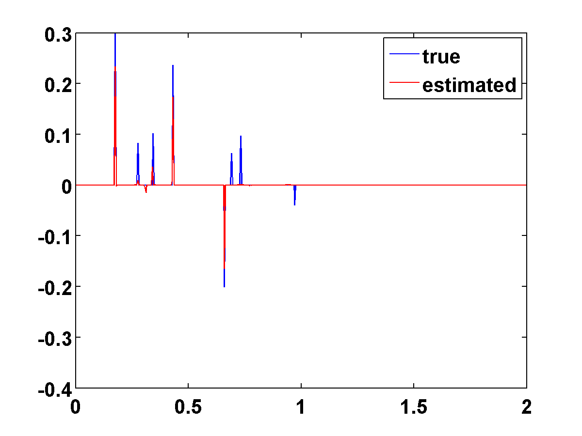
Results for the standard blind deconvolution model using \(n=5\) measurements with moderate noise (SNR \(= 13.5\)) are shown in Figure 1. There is some shift ambiguity, and for small \(n\) we found that it helps to choose \(\Gamma\) to prefer impulsive wavelets with most energy near time zero. With more measurements there is less shift ambiguity and we can typically get good results with \(\Gamma = 0\). The last two spikes are not recovered in this example is because the observed data was not long enough to see them.

EPSI Blind Deconvolution Results

Compared to the standard model, there appears to be no shift or scale ambiguity in the wavelet recovered from the EPSI model with an \(\ell_1/\ell_2\) sparsity constraint. Results for the EPSI model with \(n=50\), moderate noise (SNR \(=14.2\)) and \(\Gamma=0\) are shown in Figure 2. Despite the noise and the absence of any assumption about the support of the wavelet, both the wavelet and the largest spikes in the \(x_j\) are well recovered.

Conclusions and Future Work

We showed that a Method of Multipliers implementation of a lifted \(\ell_1/\ell_2\) constrained blind deconvolution model can be used to solve sparse blind deconvolution problems that have redundant measurements. Numerical results generally improve as the number of measurements increase. With more redundancy, more noise can be handled. The wavelet estimates are also substantially better when using the EPSI model, which doesn’t suffer from the same kind of shift and scaling ambiguities as the classical blind deconvolution model. Future work will compare to alternative approaches and other \(\ell_1/\ell_2\) implementations as well as incorporate the method into a multilevel EPSI algorithm.

Acknowledgements

This work was partly supported by the NSERC of Canada Discovery Grant (22R81254) and the Collaborative Research and Development Grant DNOISE II (375142-08). This research was carried out as part of the SINBAD II project with support from BG Group, BGP, CGG, Chevron, ConocoPhillips, Ion, Petrobras, PGS, Statoil, Sub Salt Solutions, Total SA, Woodside and WesternGeco.