Contents

% Time domain excample of constrained FWI

% Author: Mathias Louboutin using Bas Peters framework
%         Seismic Laboratory for Imaging and Modeling
%         Department of Earth, Ocean, and Atmosperic Sciences
%         The University of British Columbia
%
% Lat update: January 2016

% You may use this code only under the conditions and terms of the
% license contained in the file LICENSE provided with this source
% code. If you do not agree to these terms you may not use this
% software.

% If you have any questions, errors or disappointing results, email
% (mloubout {at} eos.ubc.ca)
close all
clear all
clc

startup

startup

current_dir = pwd;
addpath([current_dir,'/../mbin']);
cd ../results

Define general options for constraints, same as frequency domain

[constraint,options]=Default_constraints_setup();

% The following lines are the options set inside Default_constraints_setup
% You can modify it or leave it commented and us the default options

%Dykstra options
% constraint.options_dyk.maxIt=20;
% constraint.options_dyk.minIt=3;
% constraint.options_dyk.evol_rel_tol=1e-5;
% constraint.options_dyk.tol=1e-2;
% constraint.options_dyk.feas_tol=1e-1;
% constraint.options_dyk.log_feas_error=0;
% constraint.options_dyk.log_vec=0;
%
% constraint.ADMM_options.maxit=800;
% constraint.ADMM_options.evol_rel_tol=1e-6;
% constraint.ADMM_options.rho=1e2;
% constraint.ADMM_options.adjust_rho=1;
% constraint.ADMM_options.test_feasibility=0;
% constraint.ADMM_options.feas_tol=1e-2;
%
% % optimization options
%
% options.maxIter = 20;
% options.memory  = 1;
% options.testOpt = 0;
% options.verbose = 3;
% options.interp=0;
%
%
% % bound constraints
% constraint.v_max   = vpmax; %upper bound
% constraint.v_min   = vpmin; %lower bound
% constraint.v_max_plus   = 1.5; %upper bound is current highest velocity + params.v_max_plus
% constraint.v_min_minus  = .05; %lower bound is current lowest velocity -  params.v_min_minus
%
%
% %Total Variation
% constraint.TV_initial    = 4;
% constraint.TV_increment  = 2;
% constraint.TV_proj       = 'admm';
% constraint.TV_units      = 's^2/km^2';%'s^2/m^2';
% minimum smoothness    full none aspect
% constraint.smoothpars    = [4, 5, 3];%(0.8)

define velocity model

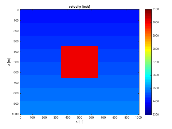
% grid
z = 0:10:1000;
x = 0:10:1000;
[o,d,n] = grid2odn(z,x);
[zz,xx] = ndgrid(z,x);

% background velocity 2500 [m/s]
v0 = linspace(2400,2500,length(z))'*ones(1,length(x));

% circular perturbation with radius 250 m and strenth 10\%
%dv = 0*xx; dv((xx-500) + (zz-500) <= 250) = .2*2500;
v = v0;
center_x = round(length(x)/2); center_z = round(length(z)/2);
v(center_z-15:center_z+15,center_x-15:center_x+15)=2500+.2*2500;

vpmin=min(v(:))-100;
vpmax=max(v(:))+100;
m=1e6./(v).^2;
m0=1e6./v0.^2;
% plot
figure;imagesc(x,z,v,[vpmin vpmax]);xlabel('x [m]');ylabel('z [m]');title('velocity [m/s]');colorbar;colormap(jet);

transmission experiment

% grid
model_t.o = [o 0];
model_t.d = [d d(1)];
model_t.n = [n 1];
model_t.space_order=4;
model_t.freesurface=0;

% Time axis
model_t.T=1500; % 1s recording
% frequencies 15 Hz Ricker wavelet.
model_t.f0 =  0.015;
[m,model_t,m0]=Setup_CFL(m,model_t,m0);
% Ricker wavelet with peak frequency f0 and phase shift t0
q=sp_RickerWavelet(model_t.f0,1/model_t.f0,model_t.dt,model_t.T);
model_t.NyqT=0:model_t.dt:model_t.T; % Data recorded at every time step
% source and receiver locations
model_t.zsrc = 0:100:1000; nsrc = length(model_t.zsrc);
model_t.xsrc = 50*ones(size(model_t.zsrc));
model_t.ysrc = 0*ones(size(model_t.xsrc));
model_t.zrec = 0:10:1000;  nrec = length(model_t.zrec);
model_t.xrec = 950;
model_t.yrec = 0;
model_t.type='full'; % Same receiver for all sources
model_t.save='RAM'; % Save forward wavefield in RAM
% create data
D_t = Gen_data(m,model_t,q);

% inversion
% create function handle for misfit
fh = @(x) GS(x,model_t,q,D_t);

Choose the constraints you want

constraint.use_bounds       = 1;
constraint.use_min_smooth   = 0;
constraint.use_TV           = 0;

Run the inversion

P = setup_constraintsTS(constraint,model_t,m0,1); %get projectors
funProj = @(input) Dykstra_prox_parallel(input,P,constraint.options_dyk); % get projector onto the intersection

[mn_t,ffinal,nfunEvals,nprojects] = minConf_PQNTS(fh,m0,funProj,options);

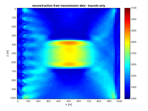
Plot the result

mn_t=reshape(1e3./sqrt(mn_t),model_t.n);

figure;imagesc(x,z,mn_t,[vpmin vpmax]);xlabel('x [m]');ylabel('z [m]');title('reconstruction from transmission data - bounds only');
colorbar;colormap(jet);

Choose the constraints you want

constraint.use_bounds       = 1;
constraint.use_min_smooth   = 0;
constraint.use_TV           = 1;

Run the inversion

P = setup_constraintsTS(constraint,model_t,m0,1); %get projectors
funProj = @(input) Dykstra_prox_parallel(input,P,constraint.options_dyk); % get projector onto the intersection

[mn_t,ffinal,nfunEvals,nprojects] = minConf_PQNTS(fh,m0,funProj,options);

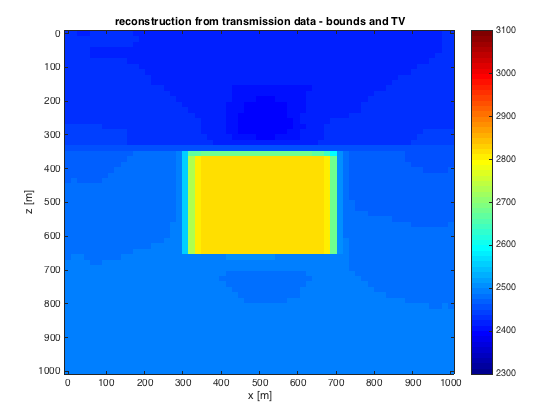
Plot the result

mn_t=reshape(1e3./sqrt(mn_t),model_t.n);

figure;imagesc(x,z,mn_t,[vpmin vpmax]);xlabel('x [m]');ylabel('z [m]');title('reconstruction from transmission data - bounds and TV');
colorbar;colormap(jet);