Contents

% Illustrates the benifit of solving constrained formulations of FWI.
% Various examples of constraints for a simple 2D model in a well-to-well
% setting. Receivers in one well, sources in the other.
%
% It should take a couple of minutes to run. To run
% in parallel, use parpool(6), because there are 6 frequencies.

% Author: Bas Peters
%         Seismic Laboratory for Imaging and Modeling
%         Department of Earth, Ocean, and Atmosperic Sciences
%         The University of British Columbia
%
% Lat update: January 2016

% You may use this code only under the conditions and terms of the
% license contained in the file LICENSE provided with this source
% code. If you do not agree to these terms you may not use this
% software.

% If you have any questions, errors or disappointing results, email
% (bpeters {at} eos.ubc.ca)

close all
clear

startup

startup

current_dir = pwd;
addpath([current_dir,'/mbin']);
cd results

Define general options for constraints

%Dykstra options (for computing the projection onto the intersection of
%multiple constraints)
constraint.options_dyk.maxIt=20;
constraint.options_dyk.minIt=3;
constraint.options_dyk.evol_rel_tol=1e-5;
constraint.options_dyk.tol=1e-2;
constraint.options_dyk.feas_tol=1e-1;
constraint.options_dyk.log_feas_error=0;
constraint.options_dyk.log_vec=0;

% ADMM options (for computing projections onto a single set in case there
% is no closed form solution)
constraint.ADMM_options.maxit=800;
constraint.ADMM_options.evol_rel_tol=1e-6;
constraint.ADMM_options.rho=1e2;
constraint.ADMM_options.adjust_rho=1;
constraint.ADMM_options.test_feasibility=0;
constraint.ADMM_options.feas_tol=1e-2;

optimization options

options.maxIter = 20;
options.memory  = 5;
options.testOpt = 0;
options.progTol=1e-14;

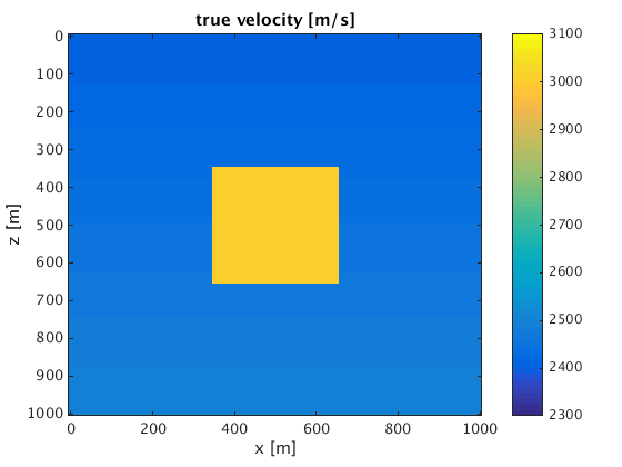
define velocity model

% grid
z = 0:10:1000;
x = 0:10:1000;
[o,d,n] = grid2odn(z,x);
[zz,xx] = ndgrid(z,x);

% background velocity 2500 [m/s]
v0 = linspace(2400,2500,length(z))'*ones(1,length(x));

% circular perturbation with radius 250 m and strenth 10\%
%dv = 0*xx; dv((xx-500) + (zz-500) <= 250) = .2*2500;
v = v0;
center_x = round(length(x)/2); center_z = round(length(z)/2);
v(center_z-15:center_z+15,center_x-15:center_x+15)=2500+.2*2500;

vpmin=min(v(:))-100;
vpmax=max(v(:))+100;

% plot
figure;imagesc(x,z,v,[vpmin vpmax]);xlabel('x [m]');ylabel('z [m]');title('true velocity [m/s]');colorbar;

set up the experiment: sources, receivers frequencies, source function

% grid
model_t.o = o;
model_t.d = d;
model_t.n = n;

% frequencies in Hz.
model_t.freq = linspace(5,15,6); nfreq = length(model_t.freq);

% Ricker wavelet with peak frequency f0 and phase shift t0
model_t.f0 = 15;
model_t.t0 = 0;

% source and receiver locations
model_t.zsrc = 0:100:1000; nsrc = length(model_t.zsrc);
model_t.xsrc = 50;
model_t.zrec = 0:10:1000;  nrec = length(model_t.zrec);
model_t.xrec = 950;

model_t.n(3)=1;
model_t.d(3)=1;
model_t.o(3)=0;

% source matrix, each column is a source function defined on the source
% grid [model.zsrc, model.xsrc].
Q = speye(nsrc);

% squared slowness [km^2/s^2]
m = 1e6./(v(:)).^2;

% initial model
m0 = 1e6./v0(:).^2;

params=[];
if isfield(params,'pdefunopts')==0
    params.pdefunopts = PDEopts2D();
end
if isfield(params,'lsopts')==0
    solve_opts = LinSolveOpts();
    solve_opts.solver = LinSolveOpts.SOLVE_LU;
    params.lsopts = solve_opts;
end

create synthetic 'observed' data

D_t = F(m,Q,model_t,params);

create function handle for misfit

%this is the only component that needs to be replaced if you want to use
%your own codes which provides a function value and gradient
%[f,g]=fh(velocity_model)

params.wri = false;
params.dist_mode = 'freq';
fh = misfit_setup(Q,D_t,model_t,params);

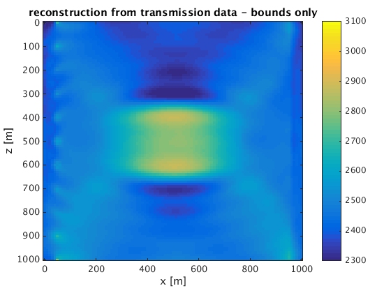
use SPG with only bound constraints

constraint.v_max   = vpmax; %upper bound
constraint.v_min   = vpmin; %lower bound

constraint.use_bounds       = 1;
constraint.use_min_smooth   = 0;
constraint.use_nuclear      = 0;
constraint.use_rank         = 0;
constraint.use_TV           = 0;
constraint.use_cardinality  = 0;
constraint.use_TD_bounds    = 0;
constraint.use_cvxbody      = 0;

params.freq_index=[1:length(model_t.freq)];
P = setup_constraints_freq_FWI_2D(constraint,model_t,model_t,params,m0,1); %get projectors
funProj =@(input) P{1}(input); %only one constraint in this case

[mn_t,fsave,funEvals,projects,iter_save] = minConf_SPG(fh,m0,funProj,options);

mn_t=1e3./sqrt(mn_t);

% plot
figure;imagesc(x,z,reshape(real(mn_t),n),[vpmin vpmax]);xlabel('x [m]');ylabel('z [m]');title('reconstruction from transmission data - bounds only');
colorbar

solve transmission experiment - bounds and Fourier based minimum smoothness

% define constraints here

%bound constraint options (all optimization methods use bound constraints)
constraint.v_max   = vpmax; %upper bound
constraint.v_min   = vpmin; %lower bound

% minimum smoothness    full none aspect
constraint.smoothpars    = [3,  3,   1];%(0.8)

constraint.use_bounds       = 1;
constraint.use_min_smooth   = 1;
constraint.use_nuclear      = 0;
constraint.use_rank         = 0;
constraint.use_TV           = 0;
constraint.use_cardinality  = 0;
constraint.use_TD_bounds    = 0;
constraint.use_cvxbody      = 0;

params.freq_index=[1:length(model_t.freq)];
P = setup_constraints_freq_FWI_2D(constraint,model_t,model_t,params,m0,1); %get projectors
funProj = @(input) Dykstra_prox_parallel(input,P,constraint.options_dyk); % get projector onto the intersection

% use SPG with constraints
[mn_t,fsave,funEvals,projects,iter_save] = minConf_SPG(fh,m0,funProj,options);
mn_t=1e3./sqrt(mn_t);

% plot
figure;imagesc(x,z,reshape(mn_t,n),[vpmin vpmax]);xlabel('x [m]');ylabel('z [m]');title('reconstruction from transmission data - bounds and Fourier minimum smoothness');

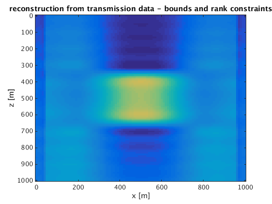
transmission experiment - Bound constraints and rank

% define constraints here

%bound constraint options (all optimization methods use bound constraints)
constraint.v_max   = vpmax; %upper bound
constraint.v_min   = vpmin; %lower bound

%rank
constraint.r_initial   = 2; %initial rank of the estimated model
constraint.r_increment = 0; %increase the rank of the estimated model by this number each new frequency batch


constraint.use_bounds       = 1;
constraint.use_min_smooth   = 0;
constraint.use_nuclear      = 0;
constraint.use_rank         = 1;
constraint.use_TV           = 0;
constraint.use_cardinality  = 0;
constraint.use_TD_bounds    = 0;
constraint.use_cvxbody      = 0;

params.freq_index=[1:length(model_t.freq)];
P = setup_constraints_freq_FWI_2D(constraint,model_t,model_t,params,m0,1); %get projectors
funProj = @(input) Dykstra_prox_parallel(input,P,constraint.options_dyk); % get projector onto the intersection

% use SPG with constraints
[mn_t,fsave,funEvals,projects,iter_save] = minConf_SPG(fh,m0,funProj,options);
mn_t=1e3./sqrt(mn_t);

% plot
figure;imagesc(x,z,reshape(mn_t,n),[vpmin vpmax]);xlabel('x [m]');ylabel('z [m]');title('reconstruction from transmission data - bounds and rank constraints');

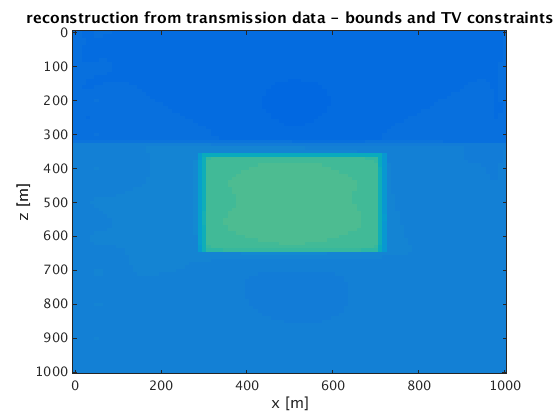
transmission experiment - Bound constraints and TV

constraint.v_max   = vpmax; %upper bound
constraint.v_min   = vpmin; %lower bound

%Total Variation
constraint.TV_initial    = 3;
constraint.TV_increment  = 1;
constraint.TV_proj       = 'admm';
constraint.TV_units      = 's^2/m^2';

constraint.use_bounds       = 1;
constraint.use_min_smooth   = 0;
constraint.use_nuclear      = 0;
constraint.use_rank         = 0;
constraint.use_TV           = 1;
constraint.use_cardinality  = 0;
constraint.use_TD_bounds    = 0;
constraint.use_cvxbody      = 0;

params.freq_index=[1:length(model_t.freq)];
P = setup_constraints_freq_FWI_2D(constraint,model_t,model_t,params,m0,1); %get projectors
funProj = @(input) Dykstra_prox_parallel(input,P,constraint.options_dyk); % get projector onto the intersection

% use SPG with constraints
[mn_t,fsave,funEvals,projects,iter_save] = minConf_SPG(fh,m0,funProj,options);
mn_t=1e3./sqrt(mn_t);

% plot
figure;imagesc(x,z,reshape(mn_t,n),[vpmin vpmax]);xlabel('x [m]');ylabel('z [m]');title('reconstruction from transmission data - bounds and TV constraints');

transmission experiment - Bound constraints and TV and rank

% define constraints here

%bound constraint options (all optimization methods use bound constraints)
constraint.v_max   = vpmax; %upper bound
constraint.v_min   = vpmin; %lower bound

%Total Variation
constraint.TV_initial    = 4;
constraint.TV_increment  = 1;
constraint.TV_proj       = 'admm';
constraint.TV_units      = 'm/s';%'s^2/m^2';

%rank
constraint.r_initial   = 2; %initial rank of the estimated model
constraint.r_increment = 0; %increase the rank of the estimated model by this number each new frequency batch

constraint.use_bounds       = 1;
constraint.use_min_smooth   = 0;
constraint.use_nuclear      = 0;
constraint.use_rank         = 1;
constraint.use_TV           = 1;
constraint.use_cardinality  = 0;
constraint.use_TD_bounds    = 0;
constraint.use_cvxbody      = 0;

params.freq_index=[1:length(model_t.freq)];
P = setup_constraints_freq_FWI_2D(constraint,model_t,model_t,params,m0,1); %get projectors
funProj = @(input) Dykstra_prox_parallel(input,P,constraint.options_dyk); % get projector onto the intersection

% use SPG with constraints
[mn_t,fsave,funEvals,projects,iter_save] = minConf_SPG(fh,m0,funProj,options);
mn_t=1e3./sqrt(mn_t);

% plot
figure;imagesc(x,z,reshape(mn_t,n),[vpmin vpmax]);xlabel('x [m]');ylabel('z [m]');title('reconstruction from transmission data - bounds, TV and rank constraints');