2D time-domain acoustic anisotropic and acoustic isotropic adjoint-state Full-waveform inversion

This is script is a basic example of time-domain full-waveform inversion on the 2D BG compass model We use gradient descent with line-search and we show the result for acoustic isotropic inversion and acoustic anisotropic inversion

Contents

Results files

result_file_ani = '../Results/m_tti_final.mat';
m_update_ani = '../Results/m_tti_update.mat';
gradient_ani = '../Results/gradient_tti.mat';
params_ani = '../Results/params_tti.mat';

result_file_iso = '../Results/m_iso_final.mat';
m_update_iso = '../Results/m_iso_update.mat';
gradient_iso = '../Results/gradient_iso.mat';
params_iso = '../Results/params_iso.mat';

read velocity [km/s], and anisotropy

load ../data/epsilon.mat;
load ../data/delta.mat;
load ../data/theta.mat;
load ../data/v0.mat;
load ../data/v.mat;

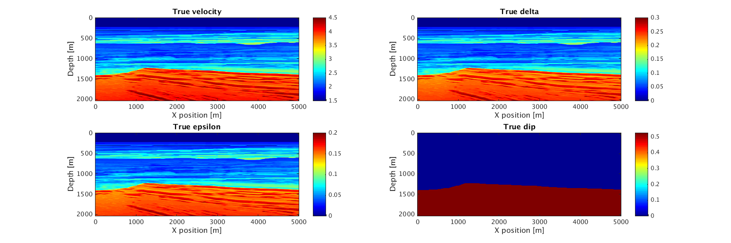
Display true models

xx=0:10:5000;
zz=0:10:2040;

hfig=figure(1);
set(hfig, 'position', [500 1200 1500 500])
subplot(2,2,1);
imagesc(xx,zz,v,[1.5 4.5]);colormap(jet);colorbar;daspect([1 1 1])
xlabel('X position [m]');
ylabel('Depth [m]');
title('True velocity');
subplot(2,2,2);
imagesc(xx,zz,delta);colormap(jet);colorbar;daspect([1 1 1])
xlabel('X position [m]');
ylabel('Depth [m]');
title('True delta');
subplot(2,2,3);
imagesc(xx,zz,epsilon);colormap(jet);colorbar;daspect([1 1 1])
xlabel('X position [m]');
ylabel('Depth [m]');
title('True epsilon');
subplot(2,2,4);
imagesc(xx,zz,theta);colormap(jet);colorbar;daspect([1 1 1])
xlabel('X position [m]');
ylabel('Depth [m]');
title('True dip');

Define initial velocity model and geometry

m=1./v.^2;
m0=1./v0.^2;
m0=reshape(m0,n);
m0(1:20,:)=m(1:20,:); % Put the real water layer
S  = opKron(opSmooth(n(2),100),opSmooth(n(1),200));  %smoothing operator
ani.delta = S*delta(:); %ones(prod(n),1)*0.3;    % values for e.g. wills point shale
ani.epsilon = S*epsilon(:); %ones(prod(n),1)*0.2;
ani.theta = S*theta(:); %ones(prod(n),1)*pi/9;

% Modeling parameters
model.o=[o 0]; %Origins of the axes [m]
model.n=[n 1]; %Number of grid points  for each dimension (excluding boundaries)
model.ddcompx=1; % Domain decomposition x direction
model.ddcompy=1; % Domain decomposition y direction
model.ddcompz=1; % Domain decomposition z direction
model.d=[d 10];
model.f0=0.015;
model.xsrc =0:100:5000;
model.zsrc= 10*ones(size(model.xsrc)); %Source coordinates along z axis [m]
model.ysrc=0*ones(size(model.xsrc));
model.xrec = (1:1:model.n(2))*model.d(2);
model.zrec=10; %Receivers coordinates along z axis [m]
model.yrec=0; %Receivers coordinates along z axis [m]
model.T=2000; %Acquisition duration [ms]
model.NyqT=0:4:model.T; % Shot record time axis [ms]
model.freesurface=0; % Freesurface ( 0 : no freesurface, 1 : freesurface)
model.space_order=4; % Space discretization order (2 or 4 only for now)
model.gppwl=6;  % grid points per wave length
model.type='full'; % Acquisitionb type is 'marine' or 'full'
% No reverse propagation of the forward wavefield to get missing time
% steps(0) or do the reverse propagation(1)
model.propag=0;
% Saving checkpints in 'RAM' or on 'disk'
model.save='RAM';
% Put the gradient to zero in the first 20 points in depth, you can also
% give an matrix of the size of the model (after CFL projection) giving the
% indexes of the physical location you don't want to update (usually waater layer or shallow part of it)
model.water=20;

Acoustic anisotropic modeling

[mm,modelm,~,anim]=Setup_CFL(m,model,[],ani);
q=sp_RickerWavelet(modelm.f0,1/modelm.f0,modelm.dt,modelm.T);
%
% dataT=Gen_data(mm,modelm,q,[],anim);

CFL conditions gives dt = 1.1985ms and d = 16  16  16 m 
Velocity interpolated on new grid

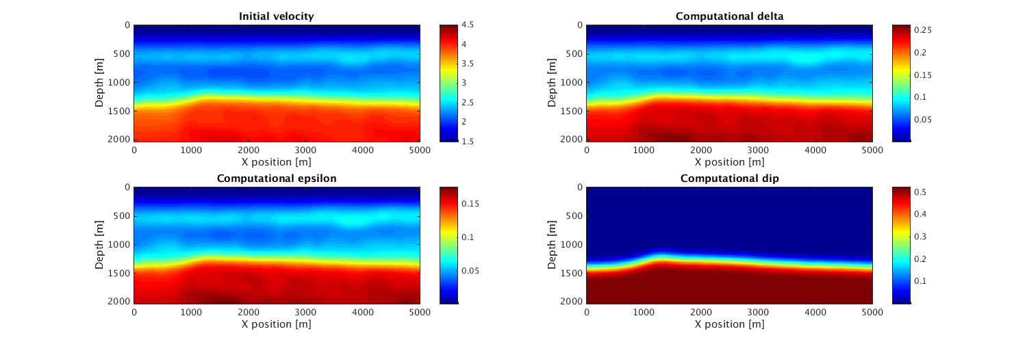
Display initial models

hfig=figure(2);
set(hfig, 'position', [500 1200 1500 500])
subplot(2,2,1);
imagesc(xx,zz,v0,[1.5 4.5]);colormap(jet);colorbar;daspect([1 1 1])
xlabel('X position [m]');
ylabel('Depth [m]');
title('Initial velocity');
subplot(2,2,2);
imagesc(xx,zz,reshape(ani.delta,model.n));colormap(jet);colorbar;daspect([1 1 1])
xlabel('X position [m]');
ylabel('Depth [m]');
title('Computational delta');
subplot(2,2,3);
imagesc(xx,zz,reshape(ani.epsilon,model.n));colormap(jet);colorbar;daspect([1 1 1])
xlabel('X position [m]');
ylabel('Depth [m]');
title('Computational epsilon');
subplot(2,2,4);
imagesc(xx,zz,reshape(ani.theta,model.n));colormap(jet);colorbar;daspect([1 1 1])
xlabel('X position [m]');
ylabel('Depth [m]');
title('Computational dip');

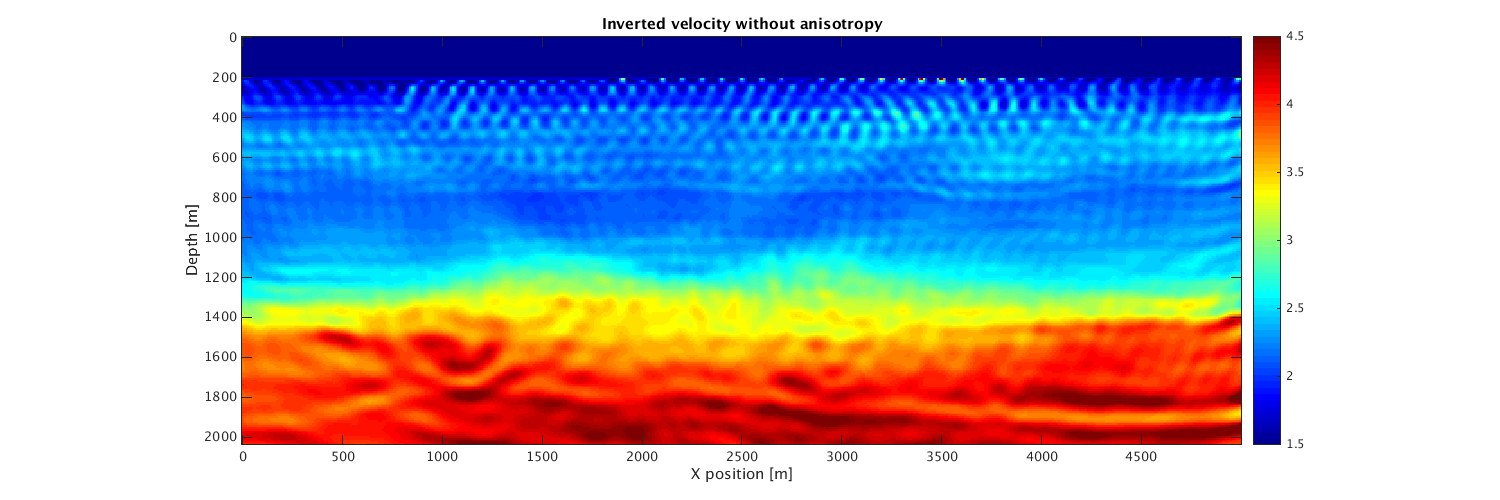
Acoustic isotropic FWI with gradient descent

[mi,modeli,mii]=Setup_CFL(m0,model,m);
modeli.water=find(sqrt(1./mii)<1.5);
q=sp_RickerWavelet(modeli.f0,1/modeli.f0,modeli.dt,modeli.T);
V_init=mi;
% nGrad=5;
% modeli.iter = nGrad;
% misfit_iso = zeros(nGrad,1);
%
% % operators for saving snapshots
% opSaveM = opSaveSnapshot(modeli.n(1)*modeli.n(2),m_update_iso);
% opSaveGradient = opSaveSnapshot(modeli.n(1)*modeli.n(2),gradient_iso);
%
% fh=@(x)GS(x,modeli,q,dataT);
%
% for i=1:nGrad
% 	fprintf('Iteration No. %d \n',i);
% 	[f0,g0]=fh(V_init);
% 	disp('f0 and g0 done starting line search');
% 	alpha=WolfeLS(fh,V_init,f0,g0,.5*min(V_init(:))/max(abs(g0(:))));
% 	g=alpha*g0;
%     V_init=V_init-g;
%
%     V_init = reshape(V_init,modeli.n);
%     gSave = reshape(g,modeli.n);
%     V_init(V_init < 1/6^2) = 1/6^2;
%     V_init(V_init > 1/1.48^2) = 1/1.48^2;
%     opSaveM*V_init(:);
%     opSaveGradient*gSave(:);
%     misfit_iso(i) = f0;
%     V_init = vec(V_init);
% end
% V_init = reshape(V_init,modeli.n);
% save(result_file_iso,'V_init','misfit_iso');
% save(params_iso,'modeli');
load(result_file_iso);
load(params_iso);
xx=0:modeli.d(2):5000;
zz=0:modeli.d(1):2040;
hfig=figure(3);set(hfig, 'position', [500 1200 1500 500])
imagesc(xx,zz,reshape(sqrt(1./V_init),modeli.n),[1.5 4.5]);colormap(jet);colorbar;daspect([1 1 1])
xlabel('X position [m]');
ylabel('Depth [m]');
title('Inverted velocity without anisotropy');

CFL conditions gives dt = 1.156ms and d = 9  9  9 m 
Velocity interpolated on new grid

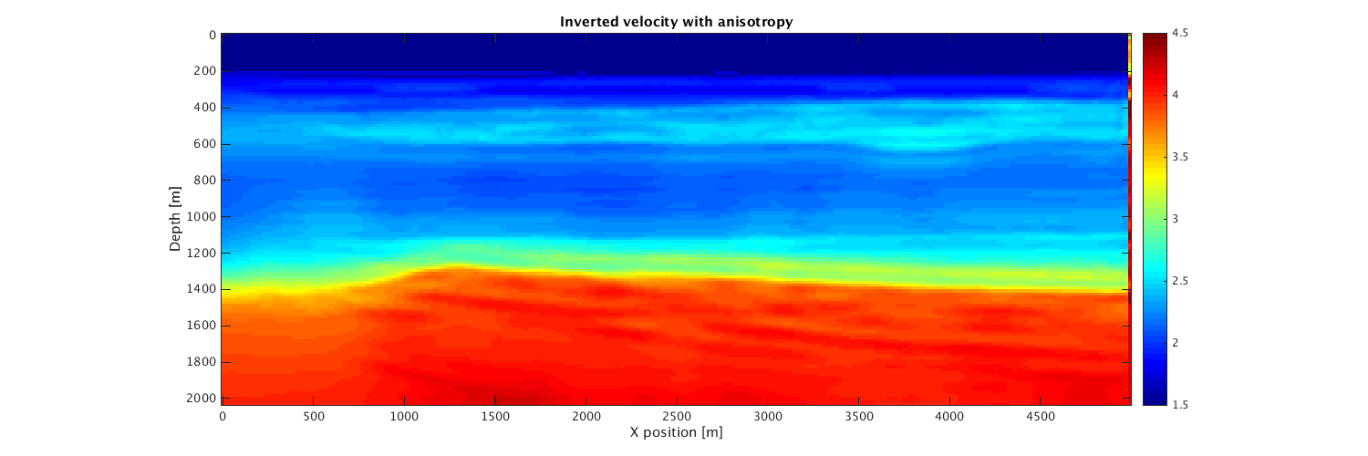
Acoustic anisotropic FWI with gradient descent

[ma,modela,maa,ania]=Setup_CFL(m0,model,m,ani);
modela.water=find(sqrt(1./maa)<1.5);
q=sp_RickerWavelet(modela.f0,1/modela.f0,modela.dt,modela.T);
V_init=ma;
% nGrad=5;
% modela.iter = nGrad;
% misfit_ani = zeros(nGrad,1);
%
% % operators for saving snapshots
% opSaveM = opSaveSnapshot(modela.n(1)*modela.n(2),m_update_ani);
% opSaveGradient = opSaveSnapshot(modela.n(1)*modela.n(2),gradient_ani);
%
% fh=@(x)GS(x,modela,q,dataT,[],ania);
%
% for i=1:nGrad
% 	fprintf('Iteration No. %d \n',i);
% 	[f0,g0]=fh(V_init);
% 	disp('f0 and g0 done starting line search');
% 	alpha=WolfeLS(fh,V_init,f0,g0,.5*min(V_init(:))/max(abs(g0(:))));
% 	g=alpha*g0;
%     V_init=V_init-g;
%
%     V_init = reshape(V_init,modela.n);
%     gSave = reshape(g,modela.n);
%     V_init(V_init < 1/6^2) = 1/6^2;
%     V_init(V_init > 1/1.48^2) = 1/1.48^2;
%     opSaveM*V_init(:);
%     opSaveGradient*gSave(:);
%     misfit_ani(i) = f0;
%     V_init = vec(V_init);
% end
% V_init = reshape(V_init,modela.n);
% save(result_file_ani,'V_init','misfit_ani');
% save(params_ani,'modela');
load(result_file_ani);
load(params_ani);
xx=0:modela.d(2):5000;
zz=0:modela.d(1):2040;
hfig=figure(4);set(hfig, 'position', [500 1200 1500 500])
imagesc(xx,zz,reshape(sqrt(1./V_init),modela.n),[1.5 4.5]);colormap(jet);colorbar;daspect([1 1 1])
xlabel('X position [m]');
ylabel('Depth [m]');
title('Inverted velocity with anisotropy');

CFL conditions gives dt = 1.3083ms and d = 16  16  16 m 
Velocity interpolated on new grid

PQN FWI via MinCon_PQN by M. Schmidt (UBC CS) with Box constraint

http://www.cs.ubc.ca/~schmidtm/Software/

You need to modify MinCon_PQN as the amplitude of the gradient are to big to work like it is. For more info to modify it

         mloubout@eos.ubc.ca

Box constraint

LB=1/(5.5^2)*ones(prod(model.n),1); UB=1/(1.45^2)*ones(prod(model.n),1); Proj=@(x)boundProject(x,LB,UB);

Gradient and objective

fh=@(x)GS(x,modela,q,dataT,[],ani);

Solve :

options.maxIter=4; options.adjustStep=0; options.verbose=3; options.corrections=5;

[m_init,f,hst,funEvals] = minConf_PQN(fh,m_init,Proj,options);