Written by Bas Peters (bpeters {at} eos.ubc.ca), September 2014.
Contents
Wavefield Reconstruction Inversion
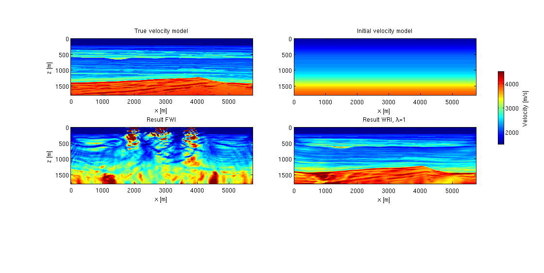
This script will show examples of waveform inversion using the BG Compass model. The theory behind this method, named Wavefield Reconstruction Inversion (WRI) is described in [1],[2] and the example shown here is based on [3].
A short overview of the method can be found at our research webpage https://www.slim.eos.ubc.ca/research/inversion#WRI
The modeling used in this example is described in https://www.slim.eos.ubc.ca/SoftwareDemos/applications/Modeling/2DAcousticFreqModeling/modeling.html.
System requirements:
- This script was tested using Matlab 2013a with the parallel computing toolbox.
- Parallelism is achieved by factorizing overdetermined systems (one for each frequency) in parallel. Each factorization requires about 15 GB.
- Runtime is about 48 hours when factorizing 5 overdetermined systems in parallel. Tested using 2.6GHz Intel processors.
Models
vr = reshape(1e3./sqrt(m_r_tmp),model.n);
vp = reshape(1e3./sqrt(m_p_tmp2),n);
v0 = reshape(1e3./sqrt(m0),n);

figWidth = 1120; % pixels
figHeight = 640;
rect = [0 50 figWidth figHeight];
figure('OuterPosition', rect)
subplot(2,2,1);set(gca,'Fontsize',10)
imagesc(x,z,v,[1500 4500]);set(gca,'plotboxaspectratio',[3.2038 1 1]);title('True velocity model')
xlabel('x [m]');ylabel('z [m]');

p=subplot(2,2,2);set(gca,'Fontsize',10)
imagesc(x,z,v0,[1500 4500]);title(['Initial velocity model'])
xlabel('x [m]');%ylabel('z [m]')
pos2=get(p,'Position');set(p,'Position',[pos2(1)-0.03 pos2(2) pos2(3) pos2(4)]);set(gca,'plotboxaspectratio',[3.2038 1 1])
pos_sub=get(p,'Position');
set(p,'Position',pos_sub)

p3=subplot(2,2,3);set(gca,'Fontsize',10)
imagesc(x,z,(vr),[1500 4500]);title('Result FWI')
xlabel('x [m]');ylabel('z [m]');
pos3=get(p3,'Position');set(p3,'Position',[pos3(1) pos3(2)+0.15 pos3(3) pos3(4)]);set(gca,'plotboxaspectratio',[3.2038 1 1])

p=subplot(2,2,4);set(gca,'Fontsize',10)
imagesc(x,z,(vp),[1500 4500]);title(['Result WRI, \lambda=',num2str(params.lambda)])
xlabel('x [m]');
pos4=get(p,'Position');set(p,'Position',[pos4(1)-0.03 pos4(2)+0.15 pos4(3) pos4(4)]);set(gca,'plotboxaspectratio',[3.2038 1 1])
pos_sub=get(p,'Position');
h = colorbar;ylabel(h, 'Velocity [m/s]','FontSize',10);
pos=get(h, 'Position');
set(h, 'Position', [pos(1)+0.08 pos(2)+0.13 0.5*pos(3) 1.53*pos(4)])
set(p,'Position',pos_sub)
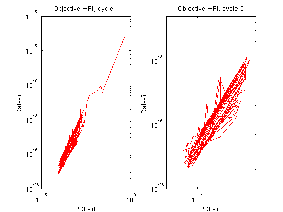
plot objectives for WRI, split up into their PDE and DATA misfit parts
figWidth = 220; % pixels
figHeight = 140;
rect = [0 50 figWidth figHeight];
figure('OuterPosition', rect)
f_p.obj_aux=reshape(f_p_tmp.obj_aux,1,length(f_p_tmp.obj_aux));
for i=1:length(f_p_tmp.obj_aux); mfp_aux_pde{i}=f_p_tmp.obj_aux{i}(:,1); end;
for i=1:length(f_p_tmp.obj_aux); mfp_aux_dat{i}=f_p_tmp.obj_aux{i}(:,2); end;
figure;
subplot(1,2,1);set(gca,'Fontsize',10);loglog(vec(cell2mat(mfp_aux_pde')),vec(cell2mat(mfp_aux_dat')),'r','LineWidth',1);
title('Objective WRI, cycle 1');xlabel('PDE-fit');ylabel('Data-fit');%pbaspect([2 1 1]);


f_p.obj_aux=reshape(f_p_tmp2.obj_aux,1,length(f_p_tmp2.obj_aux));
for i=1:length(f_p_tmp2.obj_aux); mfp_aux_pde{i}=f_p_tmp2.obj_aux{i}(:,1); end;
for i=1:length(f_p_tmp2.obj_aux); mfp_aux_dat{i}=f_p_tmp2.obj_aux{i}(:,2); end;
subplot(1,2,2);set(gca,'Fontsize',10);loglog(vec(cell2mat(mfp_aux_pde')),vec(cell2mat(mfp_aux_dat')),'r','LineWidth',1);
title('Objective WRI, cycle 2');xlabel('PDE-fit');ylabel('Data-fit');%pbaspect([2 1 1])
;axis([2e-5 2e-3 1e-10 5e-8])

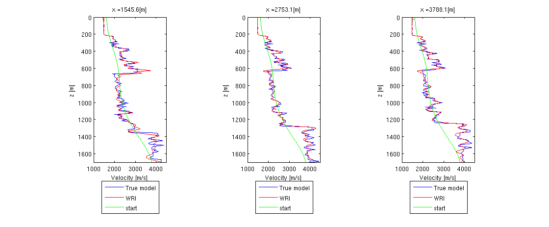
Crossections
l1=225; l2=400; l3=550;
figWidth = 1120; % pixels
figHeight = 540;
rect = [0 50 figWidth figHeight];
figure('OuterPosition', rect);set(gca,'Fontsize',10)

subplot(1,3,1);set(gca,'Fontsize',10);plot(v(:,l1),z,'LineWidth',1.5);set(gca,'YDir','reverse');hold on;title(['x =',num2str(x(l1)),'[m]']);xlabel('Velocity [m/s]');ylabel('z [m]');axis([1000 4500 0 1700]);pbaspect([0.5 1 1])
subplot(1,3,2);set(gca,'Fontsize',10);plot(v(:,l2),z,'LineWidth',1.5);set(gca,'YDir','reverse');hold on;title(['x =',num2str(x(l2)),'[m]']);xlabel('Velocity [m/s]');ylabel('z [m]');axis([1000 4500 0 1700]);pbaspect([0.5 1 1])
subplot(1,3,3);set(gca,'Fontsize',10);plot(v(:,l3),z,'LineWidth',1.5);set(gca,'YDir','reverse');hold on;title(['x =',num2str(x(l3)),'[m]']);xlabel('Velocity [m/s]');ylabel('z [m]');axis([1000 4500 0 1700]);pbaspect([0.5 1 1])

subplot(1,3,1);plot(vp(:,l1),z,'r','LineWidth',1.5);set(gca,'YDir','reverse');hold on;
subplot(1,3,2);plot(vp(:,l2),z,'r','LineWidth',1.5);set(gca,'YDir','reverse');hold on;
subplot(1,3,3);plot(vp(:,l3),z,'r','LineWidth',1.5);set(gca,'YDir','reverse');hold on;

subplot(1,3,1);plot(v0(:,l1),z,'g','LineWidth',1.5);set(gca,'YDir','reverse');
p=legend('True model','WRI','start','Location','SouthOutside');
subplot(1,3,2);plot(v0(:,l2),z,'g','LineWidth',1.5);set(gca,'YDir','reverse');
p=legend('True model','WRI','start','Location','SouthOutside');
subplot(1,3,3);plot(v0(:,l3),z,'g','LineWidth',1.5);set(gca,'YDir','reverse');
p=legend('True model','WRI','start','Location','SouthOutside');
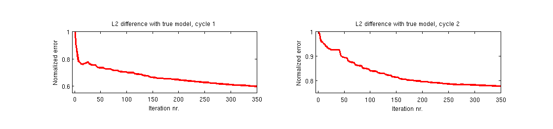
(normalized) difference with the true model
figWidth = 1120; % pixels
figHeight = 340;
rect = [0 50 figWidth figHeight];
figure('OuterPosition', rect);set(gca,'Fontsize',10)
subplot(1,2,1);set(gca,'Fontsize',10);plot(nonzeros(cell2mat(err_p_tmp)./err_p_tmp{1}(2)),'r','LineWidth',3);ylabel('Normalized error');
title('L2 difference with true model, cycle 1');xlabel('Iteration nr.');axis([-5 350 .55 1]);pbaspect([3 1 1])
subplot(1,2,2);set(gca,'Fontsize',10);plot(nonzeros(cell2mat(err_p_tmp2)./err_p_tmp2{1}(2)),'r','LineWidth',3);ylabel('Normalized error');
title('L2 difference with true model, cycle 2');xlabel('Iteration nr.');axis([-5 350 .75 1]);  pbaspect([3 1 1])
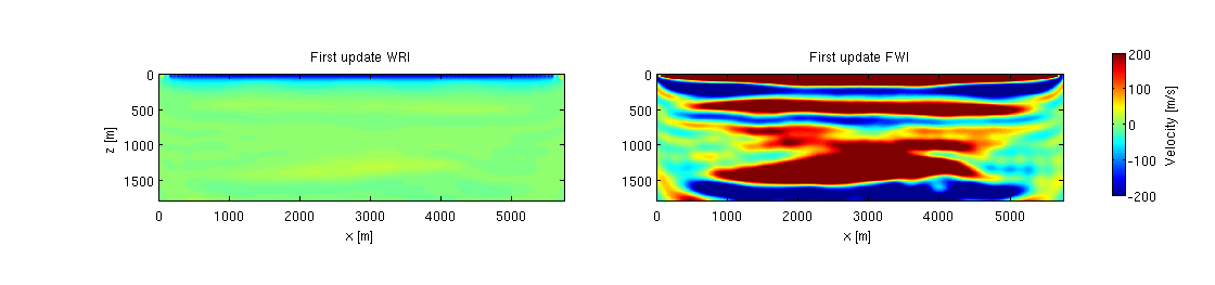
First updates for both methods at first frequency batch
figWidth = 1120; % pixels
figHeight = 340;
rect = [0 50 figWidth figHeight];
figure('OuterPosition', rect)
subplot(1,2,1);set(gca,'Fontsize',10)
imagesc(x,z,vp1-v0,[-200 200]);title('First update WRI')
xlabel('x [m]');ylabel('z [m]');axis equal tight;

p=subplot(1,2,2);set(gca,'Fontsize',10)
imagesc(x,z,vr1-v0,[-200 200]);title(['First update FWI'])
xlabel('x [m]');
pos2=get(p,'Position');set(p,'Position',[pos2(1)-0.03 pos2(2) pos2(3) pos2(4)]);axis equal tight;
pos_sub=get(p,'Position');
set(p,'Position',pos_sub)

h = colorbar;ylabel(h, 'Velocity [m/s]','FontSize',10);
pos=get(h, 'Position');
set(h, 'Position', [pos(1)+0.08 pos(2)-0.012 0.5*pos(3) 1.33*pos(4)])
set(p,'Position',pos_sub)
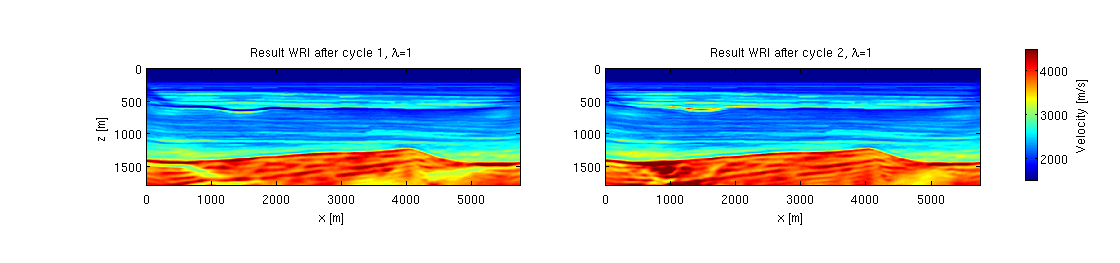
WRI model estimate after cycle 1 and cycle2 through the data
figWidth = 1120; % pixels
figHeight = 340;
rect = [0 50 figWidth figHeight];
figure('OuterPosition', rect)
subplot(1,2,1);set(gca,'Fontsize',10)
imagesc(x,z,vpc1,[1500 4500]);title(['Result WRI after cycle 1, \lambda=',num2str(params.lambda)])
xlabel('x [m]');ylabel('z [m]');axis equal tight;

p=subplot(1,2,2);set(gca,'Fontsize',10)
imagesc(x,z,vpc2,[1500 4500]);title(['Result WRI after cycle 2, \lambda=',num2str(params.lambda)])
xlabel('x [m]');
pos2=get(p,'Position');set(p,'Position',[pos2(1)-0.03 pos2(2) pos2(3) pos2(4)]);axis equal tight;
pos_sub=get(p,'Position');
set(p,'Position',pos_sub)

h = colorbar;ylabel(h, 'Velocity [m/s]','FontSize',10);
pos=get(h, 'Position');
set(h, 'Position', [pos(1)+0.08 pos(2)-0.012 0.5*pos(3) 1.33*pos(4)])
set(p,'Position',pos_sub)
References
[1] Tristan van Leeuwen, Felix J. Herrmann, Geophysical Journal International,2013. Mitigating local minima in full-waveform inversion by expanding the search space.
[2] Tristan van Leeuwen, Felix J. Herrmann. 2013. A penalty method for PDE-constrained optimization.
[3] Bas Peters, Felix J. Herrmann, Tristan van Leeuwen. EAGE, 2014. Wave-equation based inversion with the penalty method: adjoint-state versus wavefield-reconstruction inversion.