Summary of TV WRI MATLAB Code
Included files
Main Script and Functions
- main.m
- setup_problem.m
- pTV.m
- convex_sub.m
Additional Functions
- getDiscreteLap.m
- generateData.m
- getDiscreteGrad.m
- proj_TVbounds.m
- vsmooth.m
- figadust.m
- make_movie.m
Structure of Code and Summary of Algorithm
The main script is main.m and can be run by typing main at the MATLAB prompt. It calls
[model,pm,Ps,Pr,q,d,ssW] = setup_problem(example);to define a struct of model parameters, model, a struct of algorithm parameters, pm, sampling operators Ps and Pr that project onto source and receiver locations respectively, Fourier coefficients of the source wavelet q at the sampled frequencies and a cell structure of data, d, such that d{v} is a frequency slice of data at the frequency indexed by v. It also defines a matrix of weights ssW that can be used to blend sources and data to simulate simultaneous shots.
A detailed description of the total variation regularized Wavefield Reconstruction Inversion method can be found in the technical report at https://www.slim.eos.ubc.ca/content/scaled-gradient-projection-method-total-variation-regularized-full-waveform-inversion and the SINBAD presentation at https://www.slim.eos.ubc.ca/content/scaled-gradient-projection-method-total-variation-regularized-full-waveform-inversion-0. Briefly, it is minimizing a constrained quadratic penalty objective for acoustic full waveform inversion that has the form \[ \begin{equation} \label{QP} \min_m F(m) \qquad \text{s.t.} \qquad m_i \in [b_i , B_i] \text{ and } \|m\|_{TV} \leq \tau \ . \end{equation} \] where \[ \begin{equation} \label{F} F(m) = \sum_{sv}F_{sv}(m) \end{equation} \] and \[ \begin{equation} \label{Fsv} F_{sv}(m) = \frac{1}{2}\|P \bar{u}_{sv}(m) - d_{sv}\|^2 + \frac{\lambda^2}{2}\|A_v(m)\bar{u}_{sv}(m) - q_{sv}\|^2 \ . \end{equation} \] This nonconvex objective is a sum of squares of data misfits and PDE misfits in the frequency domain, summed over source indices \(s\) and frequency indices \(v\).
A candidate initial model minit is defined in setup_problem.m, but if it doesn’t satisfy the bound and TV constraints, it is projected onto the nearest model that does by calling the function proj_TVbounds.m.
minit = proj_TVbounds(minit,.99*pm.tau,model.h,pm.dpw,model.mmin,model.mmax);The resulting initial model is stored in a 3D matrix mb that will eventially contain the models (slowness squared) that are estimated after each small batch of frequency data moving from low to high frequencies in overlapping batches.
mb(:,:,1) = minit; For each frequency batch b, only a subset of frequency indices Vb are used so that the objective we work with is defined by
\[
\begin{equation}
\label{FVb}
F(m) = \sum_{s,v \in V_b}F_{sv}(m)
\end{equation}
\]
The result from the previous batch mb(:,:,b) is used as a warm start when solving the problem on the next frequency batch for mb(:,:,b+1). This procedure is carried out in main.m with the loop
for b = 1:model.batches
    [mTV,energy,oits,cinit] = pTV(model,pm,b,mb(:,:,b),Ps,Pr,q,d,ssW,cinit);
    mb(:,:,b+1) = mTV;
end
The function pTV.m solves (\(\ref{FVb}\)) by a sequence of outer iterations of the form
\[
\begin{equation}
\label{pTVb}
\begin{aligned}
\dm & = \arg \min_{\dm} \dm^T \nabla F(m^n) + \frac{1}{2}\dm^T (H^n + c_n\I) \dm \\
& \text{s.t. } m^n_i + \dm_i \in [b_i , B_i] \text{ and } \|m^n + \dm\|_{TV} \leq \tau \\
m^{n+1} & = m^n + \dm \ .
\end{aligned}
\end{equation}
\]
At the current model estimate \(m^n\), it uses the gradient \(\nabla F(m^n)\) and a diagonal Gauss Newton approximation to the Hessian \(H_n\) to construct a quadratic approximation to the objective, which can then be minimized subject to the bound and TV constraints to get a model update \(\dm\).
Inside pTV.m is a function computeGradient(), which computes the objective, the gradient and the Gauss Newton Hessian via
[obj,g,H] = computeGradient(m,model,pm,Q,ssW,Ps,Pr,freq_ind,freq,q,d);The convex subproblems for \(\dm\) are solved by an iterative primal dual method defined in the function convex_sub(), which is called by pTV.m during every outer iteration via
dm = reshape(convex_sub(model,pm,m,g,Hc),n(1),n(2));At the end of main.m, the sequence of model estimates stored in mb can be used to make a movie of the algorithm’s progress by
make_movie
movie(99,velocity_movie,1,4);
How to Modify Code to Run Different Examples
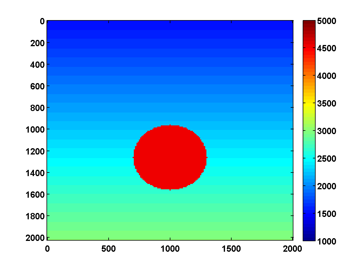
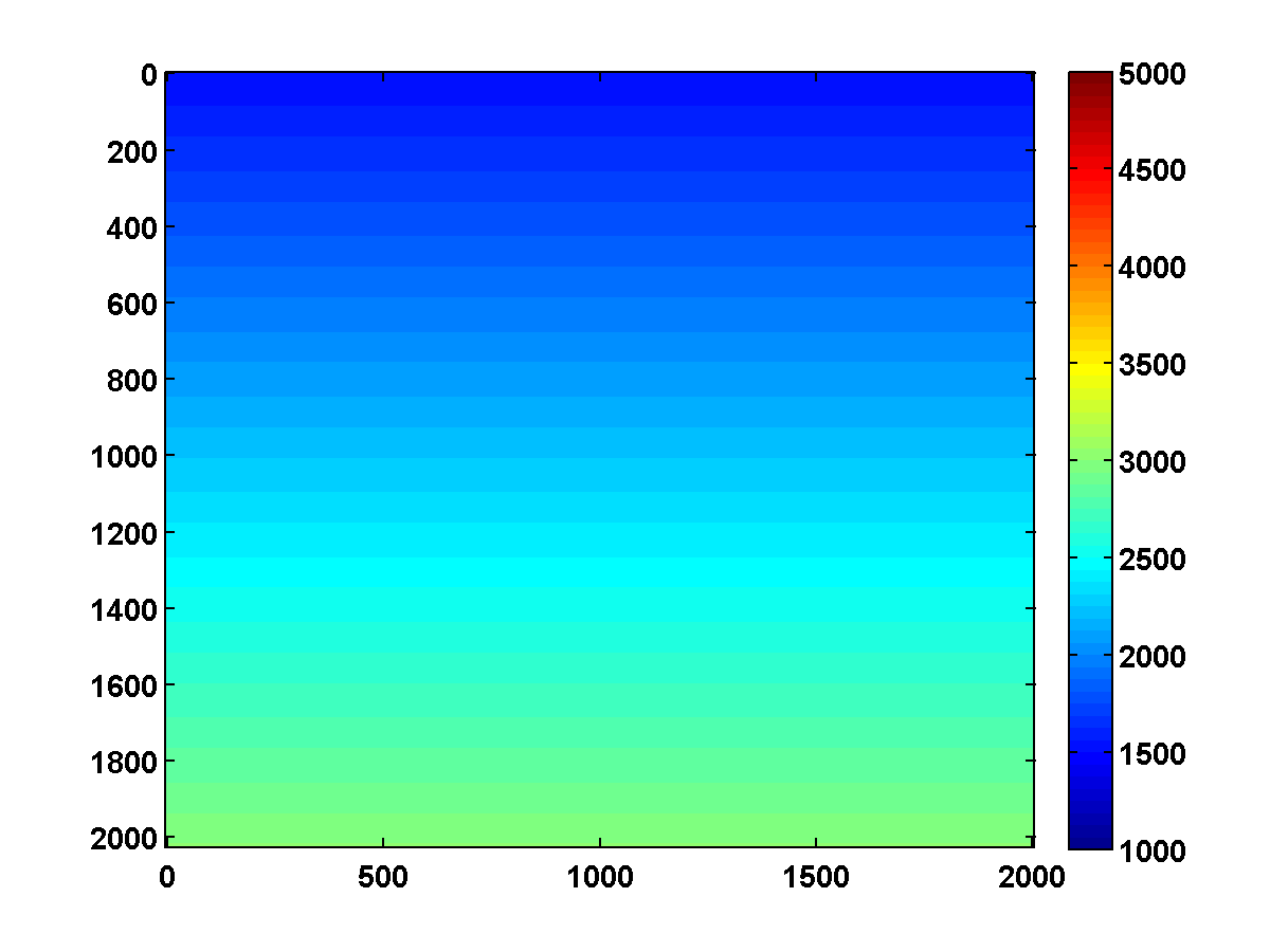
Two included examples can be run by typing main at the MATLAB prompt. In main.m set example = 'blob' to run a simple example based on a synthetic velocity model that has a high velocity blob against a smooth background velocity that increases linearly with depth. This model is defined in setup_problem.m and does not require any additional data to be downloaded. Set example = 'BPC' to use a downsampled portion of the BP 2004 Velocity Benchmark data set as the true velocity model.
Additional examples can be defined in setup_problem.m, which is currently organized as a switch statement
switch example
    case {'blob'}
        %sets up parameters and data for blob example
    case {'BPC'}
        %sets up parameters and data for BP example
end
More examples can be included as additional cases. The following parameter, data and functions are defined in setup_problem(example)
model.example = examplemodel.h– mesh width in metersmodel.n– model dimensions, depth by widthmodel.N– total number of model parameters (defined byprod(n))model.zt = 0:h:h*(n(1)-1)– \(z\) coordinatesmodel.xt = 0:h:h*(n(2)-1)– \(x\) coordinatesmodel.vtrue– define to be true velocity modelmodel.vinit– define to be initial velocity modelmodel.vmin– minimum velocity (same dimension as model)model.vmax– maximum velocity (same dimension as model)model.mtrue = 1./model.vtrue.^2model.minit = 1./model.vinit.^2model.mmin = 1./model.vmax.^2model.mmax = 1./model.vmin.^2model.freq– list of sampled frequencies (Hz)model.nf– number of frequencies usedmodel.Vb– each row defines a frequency batch by specifying the indices intomodel.freqto be used in that batchmodel.batches = size(model.Vb,1)model.f0– peak frequency of source wavelet, assumed here to be a Ricker waveletmodel.t0– phase shift of source wavelet in secondsmodel.zsrc– \(z\) coordinates of source locationsmodel.xsrc– \(x\) coordinates of source locationsmodel.ns– number of sourcesmodel.zrec– \(z\) coordinates of receiver locationsmodel.xrec– \(x\) coordinates of receiver locationsmodel.nr– number of receiversq– Fourier coefficients of the source wavelet at the sampled frequenciesmodel.vweights– optional frequency dependent weights to scale each \(F_{sv}(m)\) component of the objectivemodel.nsim– number of simultaneous shotsmodel.redraw–1to randomly redraw weights,0for no redrawsmodel.rngshots = rng('shuffle')– store seed for random number generatorssW– matrix of weights that can be used to blend sources and data to simulatemodel.nsimsimultaneous shots. Ifmodel.redraw = 1, these are redrawn from a Gaussian distribution every time the model is updated. Ifmodel.redraw = 0, the weights inssWdon’t change. The case of sequential shots corresponds to settingmodel.nsim = ns,model.redraw = 0andssW = speye(ns,model.nsim).PsandPr– sampling operators that project onto source and receiver locations. Their definitions currently assume that these locations correspond to points in the discretization.model.Xintandmodel.Xbnd– masks used in defining the absorbing boundary condition, which here is a simple Robin boundary conditionmodel.L– Discrete Laplacian defined byL = getDiscreteLap(n,h), which uses a simple \(5\) point stencilmodel.rngnoise = rng('shuffle')– store seed for random number generatormodel.dsig– if nonzero, then frequency dependent Gaussian random noise is added to the data with standard deviationmodel.dsig/sqrt(model.ns*model.nr)times the norm of each frequency slice of datad{v}model.M = @(ff,mm) (2*pi*ff)^2*spdiags(model.Xint(:).*mm(:),0,N,N) - ...1i*(2*pi*ff)*spdiags(model.Xbnd(:).*sqrt(mm(:)),0,N,N)– this function of frequency and model is used in the definition of the Helmholtz operatorL + Md– data defined bygenerateData(model,q,Ps,Pr)model.Dandmodel.Eare defined by[D,E] = getDiscreteGrad(n(1),n(2),h,pm.dpw)and used to define the TV constraintpm.dpw– optional depth weights to make the strength of the TV penalty depth dependent. Should be a vector of lengthmodel.n(1)with values between \(0\) and \(1\).pm.TV = @(t) sum(sqrt(E'*((D*t(:)).^2)))– function for evaluating the total variation of amodel.n(1)bymodel.n(2)image.pm.mu– numerical parameter that doesn’t change objective but can affect rate of convergence. OK to set to \(1\).pm.lambda– penalty parameter for PDE misfitpm.tau– parameter for total variation constraint. The total variation of the true model ispm.TV(model.mtrue)pm.cminandcmax– bounds on an adaptive parameter for damping the Hessianpm.c1– factor to decrease c if objective is decreasing enoughpm.c2– factor to increase c if objective doesn’t decrease enoughpm.sigma– what fraction of ideal objective decrease is acceptablepm.itol– tolerance for inner iteration stopping conditionpm.miniits– minimum number of inner iterationspm.maxiits– maximum number of allowed inner iterationspm.admax = h^2/8– lower bound for \(\frac{1}{\|D^TD\|}\), used to define convex subproblem parameterspm.otol– tolerance for outer iteration stopping conditionpm.maxoits– maximum number of allowed outer iterationspm.minoits = min(2,pm.maxoits)– minimum number of outer iterations
Results for Included Examples
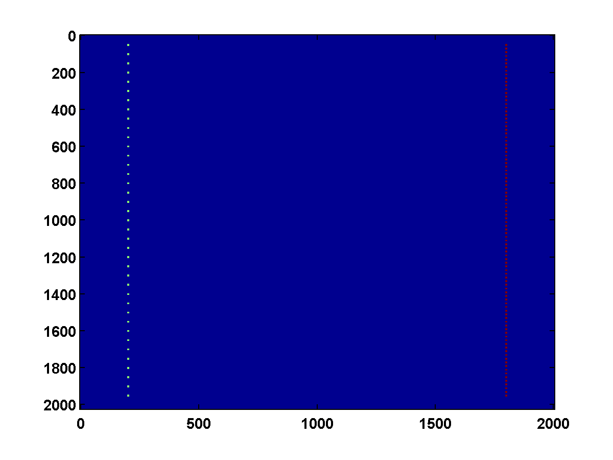
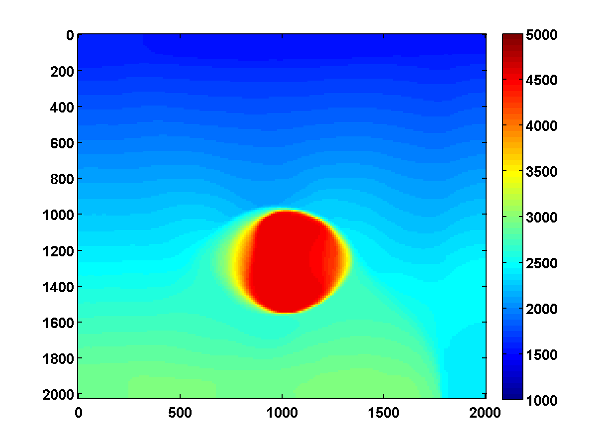
For the blob example, the true model, source and receiver locations and initial model are shown in Figure 1.
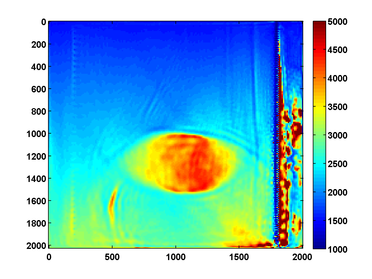
The results with \(\tau = 1000||m_{\text{true}}|_{TV}\) and \(\tau = .875||m_{\text{true}}|_{TV}\) are shown in Figure 2. Both examples use noisy data corresponding to model.dsig = .05.
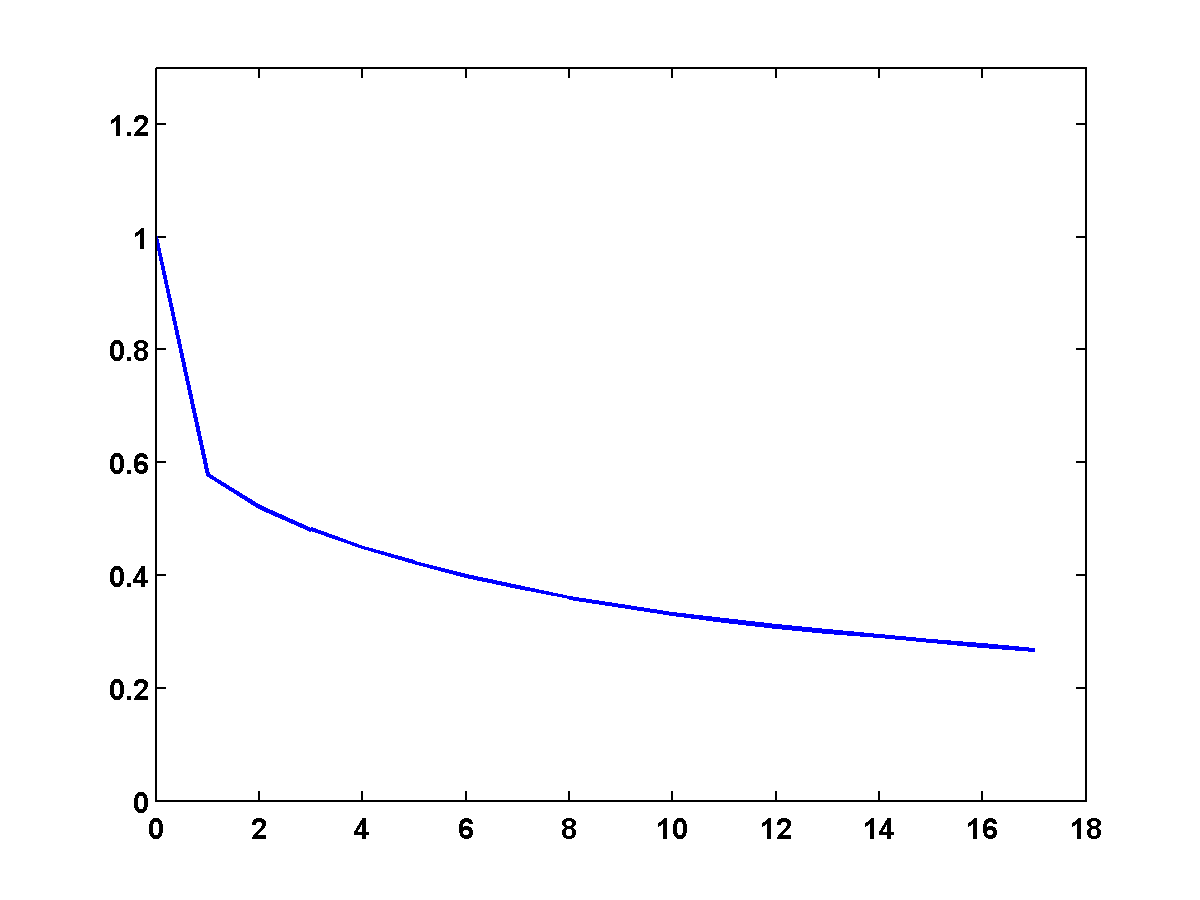
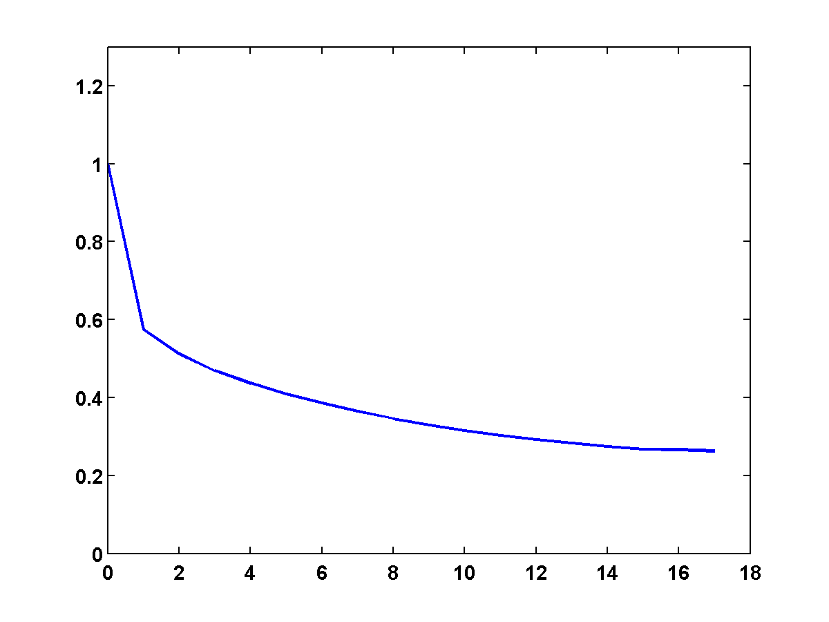
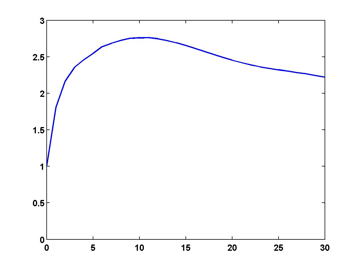
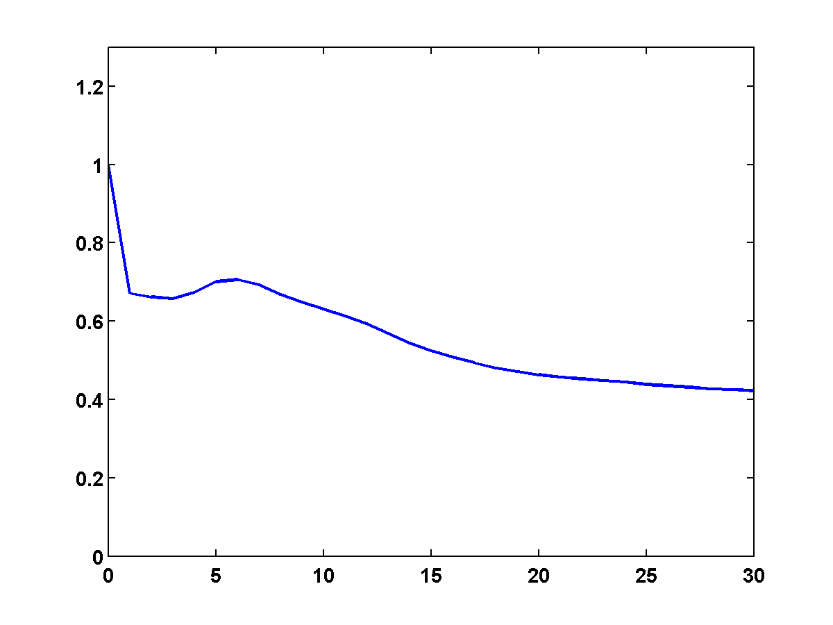
A comparison of their relative model errors are shown in Figure 3.
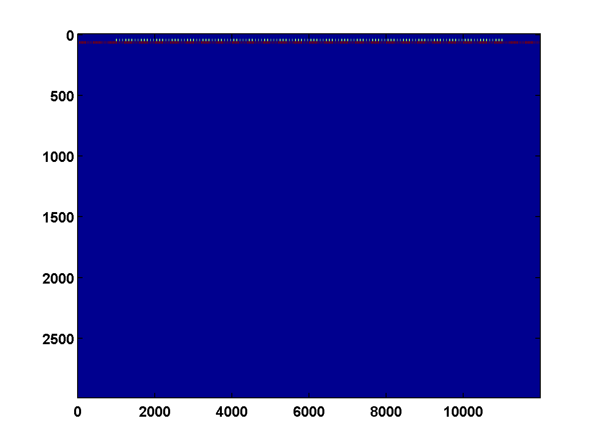
For the BP example, the true model, source and receiver locations and initial model are shown in Figure 4.

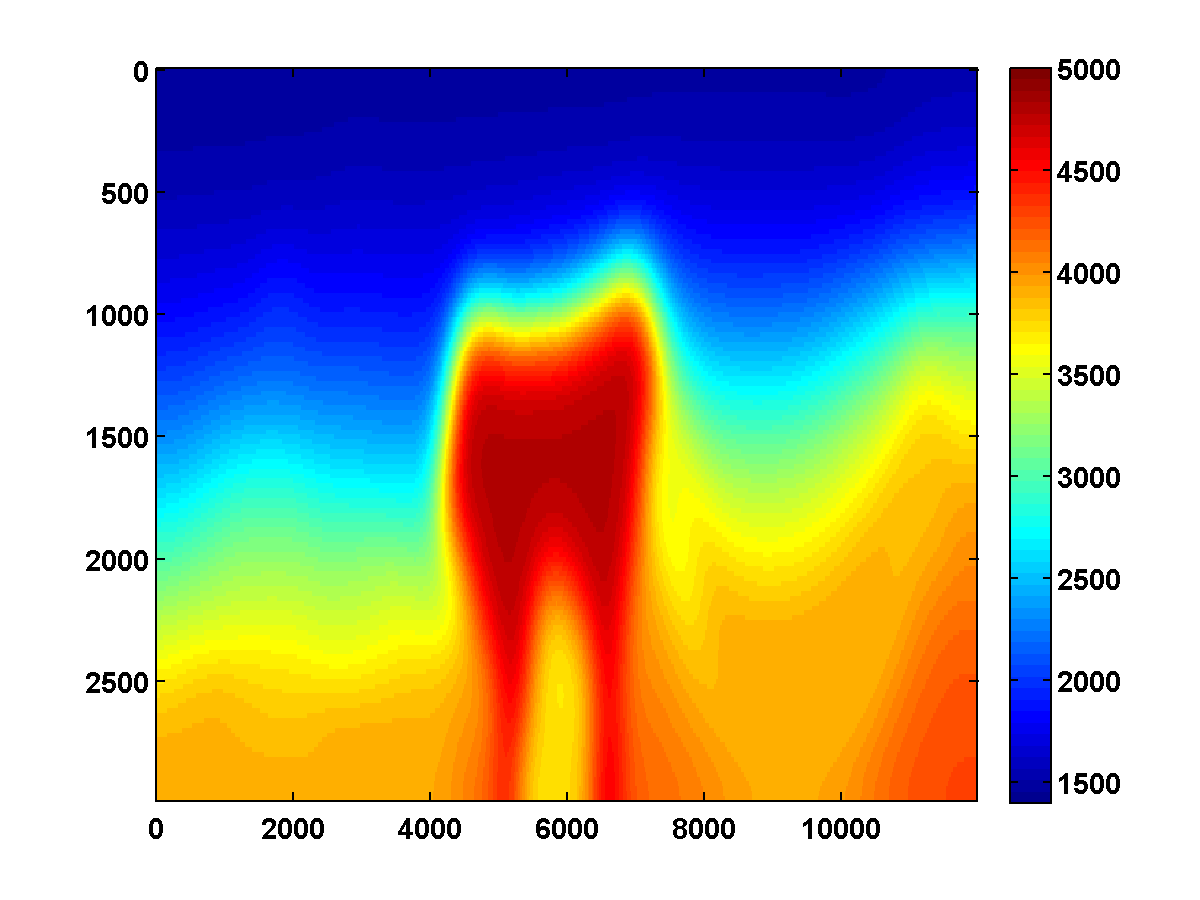
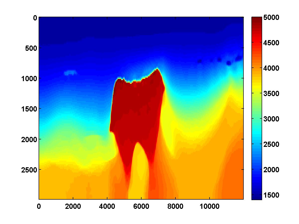
The results with \(\tau = 1000||m_{\text{true}}|_{TV}\) and \(\tau = .9||m_{\text{true}}|_{TV}\) are shown in Figure 5. Both examples use noise free synthetic data.

A comparison of their relative model errors are shown in Figure 6.