Written by Zhilong Fang (zfang@eoas.ubc.ca), March 2018.

Contents

Wavefield Reconstruction Inversion with Source Estimation

This script will show examples of waveform inversion with source estimation using the Camembert model. The theory behind this method, named Wavefield Reconstruction Inversion (WRI) with source estimation is described in [1].

The modeling used in this example is described in https://www.slim.eos.ubc.ca/SoftwareDemos/applications/Modeling/2DAcousticFreqModeling/modeling.html.

System requirements:

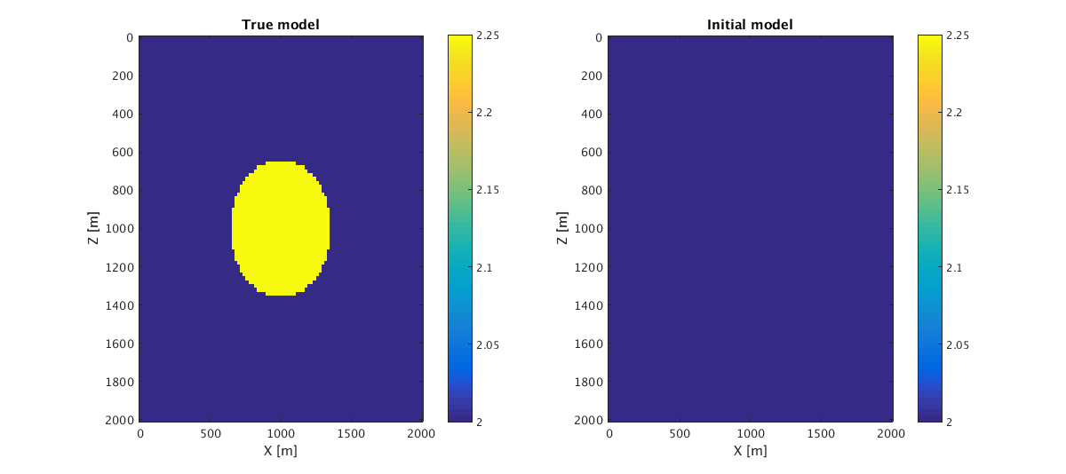
Models

  n = [101, 101];
  d = [20, 20];
  o = [0, 0];

  vel    = 2*ones(n);
  velini = vel;
  for i = 1:n(1)
    for j = 1:n(2)
      if norm([i-51,j-51])<18
          vel(i,j) = 2.25;
      end
    end
  end
%
  model.zsrc = d(1):d(1)*2:d(1)*(n(1)-2);
  model.xsrc = d(1)*2;
  model.zrec = d(1):d(1):d(1)*(n(1)-2);
  model.xrec = d(1)*(n(1)-2);

  [zz xx] = odn2grid(o,d,n);

% The true model and initial model are
  figure;subplot(1,2,1)
  imagesc(zz,xx,vel);xlabel('X [m]');ylabel('Z [m]');a =caxis;colorbar
  title('True model')

  subplot(1,2,2)
  imagesc(zz,xx,velini);xlabel('X [m]');ylabel('Z [m]');caxis(a);colorbar
  title('Initial model')
  x0=10;
  y0=10;
  width=900;
  height=400;
  set(gcf,'units','points','position',[x0,y0,width,height])

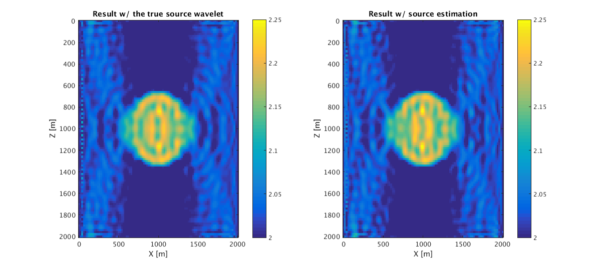
Inversion result

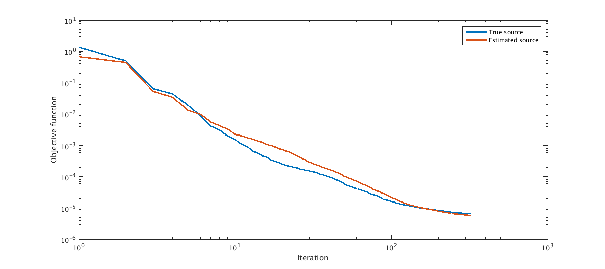
%The inversion results w/ the true source wavelet and w/ the source estimation are:

  load('../results/Result_truesrc.mat');
  m_t = Result.mf;
  v_t = reshape(1./sqrt(m_t),n);
  info_t = Result.info;
  info_t = info_t.obj;

  figure;subplot(1,2,1)
  imagesc(zz,xx,v_t);xlabel('X [m]');ylabel('Z [m]');caxis(a);colorbar
  title('Result w/ the true source wavelet')

  load('../results/Result_estsrc.mat');
  m_e = Result.mf;
  v_e = reshape(1./sqrt(m_e),n);
  info_e = Result.info;
  info_e = info_e.obj;

  subplot(1,2,2)
  imagesc(zz,xx,v_e);xlabel('X [m]');ylabel('Z [m]');caxis(a);colorbar
  title('Result w/ source estimation')
  x0=10;
  y0=10;
  width=900;
  height=400;
  set(gcf,'units','points','position',[x0,y0,width,height])

%The comparison of the objective history is:

  nit    = min(length(info_e),length(info_t));
  info_e = info_e(:);
  info_t = info_t(:);
  xi     = [1:nit];
  xi     = xi(:);
  figure;loglog(xi, [info_t(1:nit) info_e(1:nit)],'linewidth',2);
  xlabel('Iteration');ylabel('Objective function');
  legend('True source','Estimated source')
  x0=10;
  y0=10;
  width=900;
  height=400;
  set(gcf,'units','points','position',[x0,y0,width,height])

%The compaison of the source wavelet is shown as follows.

%The true source function is

  load('../results/src_true.mat');
  src_true

%The estimated source function is
  load('../results/src_est.mat');
  src_est

src_true =

    3.5794   13.2437    6.2177


src_est =

   3.5810 - 0.0206i  13.1653 - 0.1947i   6.1422 - 0.1137i

References

[1] Zhilong Fang, Rongrong Wang. Felix J. Herrmann, 2017, Source estimation for wavefield-reconstruction inversion.