Fast Robust Waveform inversion: functions

The functions specific to this package can be found in the mbin directory.

• twonorms - the two-norm and its derivative.
• hubers - the Huber misfit and its derivative.
• hybrid - the hybrid misfit and its derivative.
• students - the Students t misfit and its derivative.
• Jls - least-squares residual and gradient for given model and observed data.
• JW - sim. source misfit and gradient for given model and observed data.
• JI_src - misfit and gradient for subset of sources
• mylbfgs - standard L-BFGS with Wolfe linesearch
• lbfgsbatch - L-BFGS that works on a different subset of the sources at each iteration.

Contents

Penalty functions

The penalty functions are of the form

$f(\mathbf{r}) = \sum_i p(r_i)$,

where

$p(r) = \frac{1}{2}r^2$

for least-squares,

$p(r) = \frac{1}{2\epsilon}r^2 \quad \mathrm{for} \quad | r |\leq \epsilon \quad \mathrm{and} \quad | r |-\epsilon/2 \quad \mathrm{otherwise}$

for the Huber,

$p(r) = \sqrt{1 + | r |^2/\epsilon} - 1$

for the hybrid [1], and

$p(r) = \log(1 + | r |^2/k)$

for Students t.

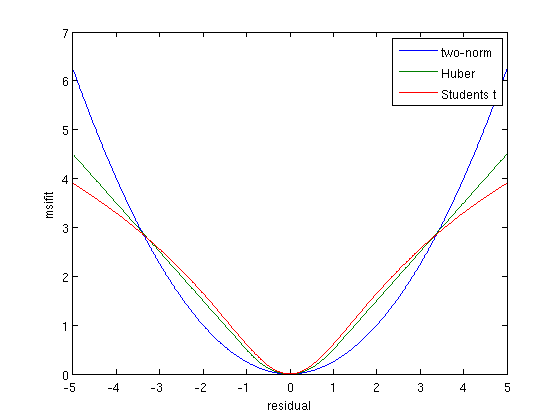
The functions twonorms, hubers, hybrid and students calculate the misfit and its gradient for a given residual vector. The penalties look like this.

% residual vector
r = [-5:.01:5];

% evaluate on scalar residual
for k = 1:length(r)
    ls(k) = .5*twonorms(r(k));
    hb(k) = hubers(r(k));
    st(k) = students(r(k));
end

% plot
figure;
plot(r,ls,r,hb,r,st);
xlabel('residual');ylabel('msifit');legend('two-norm','Huber','Students t');

Misfit functions for FWI

Based on the above penalty functions, we can calculate the misfit for FWI, given a model $\mathbf{m}$ and observed data $\mathbf{d}_i$:

$J(\mathbf{m}) = \sum_i f(F(\mathbf{m})\mathbf{q}_i - \mathbf{d}_i)$,

where $F(\mathbf{m})\mathbf{q}_i$ is the modeled data for the $i$-th source.

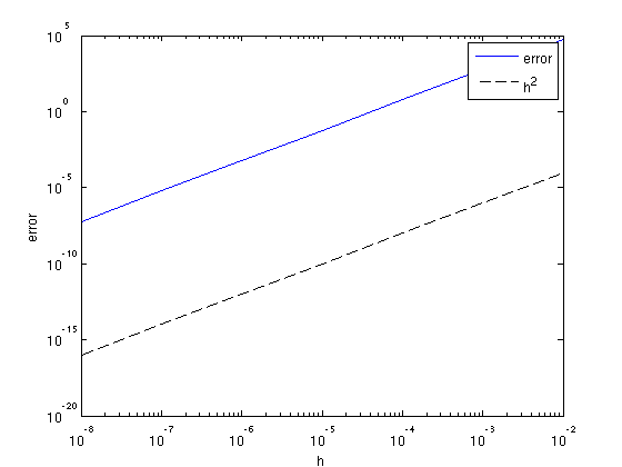
We can test the accuracy of the gradient based on the Taylor series:

$J(\mathbf{x} + h\Delta \mathbf{x}) = J(\mathbf{x}) + h\nabla J(\mathbf{x})^T\Delta\mathbf{x} + \mathcal(O)(h^2)$

We can plot the error

$| J(\mathbf{x}+h\Delta\mathbf{x}) - J(\mathbf{x}) - h\nabla J(\mathbf{x}+h\Delta\mathbf{x})^T\Delta\mathbf{x} |$

as a function of $h$ and verify that it decreases as $h^2$:

% setup some model parameters
model.o = [0 0];
model.d = [10 10];
model.n = [51 51];
model.nb = [50 50];
model.freq = [10];
model.f0 = 10;
model.t0 = 0.01;
model.zsrc = 15;
model.xsrc = 0:100:1000;
model.zrec = 10;
model.xrec = 0:20:1000;

% constant velocity 2000 m/s
v0 = 2000;
m  = 1e6/v0.^2*ones(prod(model.n),1);

% random perturbation
dm = randn(prod(model.n),1);

% define point sources and make data
Q = speye(length(model.xsrc));
D = F(m,Q,model);

% define function-handle for misfit
fh = @(x)Jls(x,Q,D,model);

% test for range of h
h = 10.^[-2:-1:-8];
f0 = fh(m);
for k = 1:length(h)
    [f1, g1] = fh(m + h(k)*dm);
    e(k) = abs(f1 + h(k)*g1'*dm - f0);
end

% plot error
figure;
loglog(h,e,h,h.^2,'k--');
xlabel('h');ylabel('error');
legend('error','h^2');

Alternatively, we can check whether

$\frac{1}{2}(\nabla J(\mathbf{x}_1 + \nabla J(\mathbf{x}_2))^T(\mathbf{x}_2 - \mathbf{x}_1) = J(\mathbf{x}_2) - J(\mathbf{x_1})$

for small $| \mathbf{x}_2 - \mathbf{x}_1 |$.

m1 = m + 1e-3*randn(prod(model.n),1);
m2 = m + 1e-3*randn(prod(model.n),1);

[f1,g1] = fh(m1);
[f2,g2] = fh(m2);

.5*(g1 + g2)'*(m2 - m1)/(f2 - f1)

ans =

    1.0019

Optimization

Included are a standard L-BFGS with a Wolfe linesearch, mylbfgs.m (cf. [2]) and a modified L-BFGS that works on a different subset of the sources at each iteration, lbfgsbatch.m, see [3]

References

[1] K.P. Bube and R.T. Langan, 1997. Hybrid l1/l2 minimization with applications to tomography. Geophysics, 62, 1183–1195

[2] J. Nocedal and S.J. Wright, 1999. Numerical Optimization. Springer.

[3] M.P. Friedlander, M.Schmidt, 2011. Hybrid Deterministic-Stochastic Methods for Data Fitting. arXiv:1104.2373.