2D time-stepping Gauss-Newton full-waveform inversion (applied to Chevron 2014 benchmark dataset)

       Seismic Laboratory for Imaging and Modeling
       Department of Earch & Ocean Sciences
       The University of British Columbia

Contents

Chevron 2014 SEG FWI workshop benchmark

This is an demonstration of our workflow of time domain Gauss-Newton FWI for the benchmark dataset

Released initial model and frequency domain GN FWI result.

In this section, we carried a frequency domain GN FWI with the chevron released initial model from 3Hz to 5Hz. For more information about frequency domain GN FWI, please see [1,2]. The related code can be found in the SLIM software release under /applications/WaveformInversion/2DModGaussNewton.

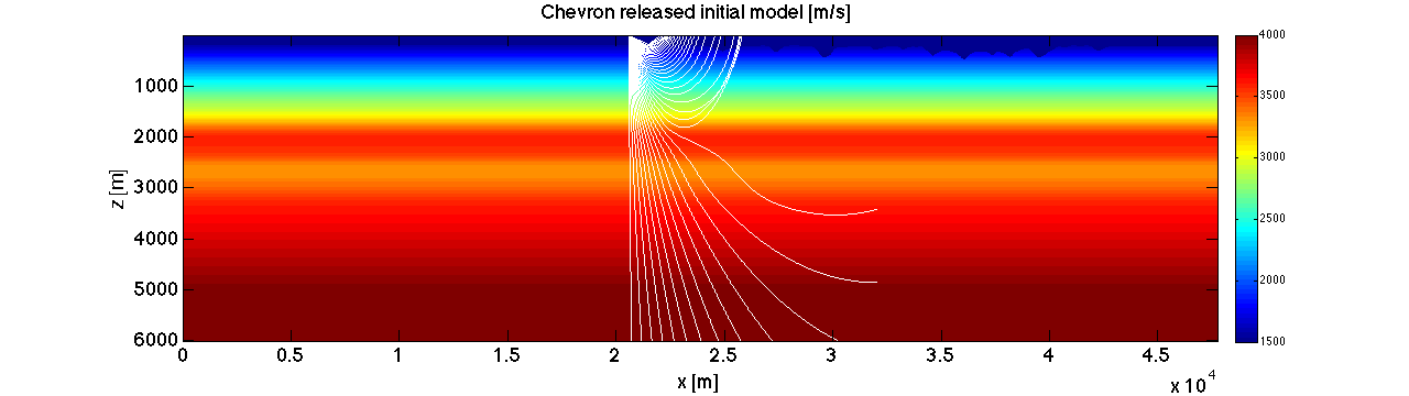
load released_model.mat
scrsz = get(0,'ScreenSize');
figure('Position',[1 scrsz(4)/4 scrsz(3)/2 scrsz(4)/4]);set(gca,'fontsize',18);
imagesc(mmx,mmz,vel_init);caxis([1500,4000]);xlabel('x [m]');ylabel('z [m]');title('Chevron released initial model [m/s]');colorbar;
load ray_paths.mat
for k=1:size(r1,1)
	r = r1{k};
	line(r(:,1)+20000,r(:,2),ones(size(r,1)),'color','w','lineWidth',1);
end

load model_freq_forfwi.mat
scrsz = get(0,'ScreenSize');
figure('Position',[1 scrsz(4)/4 scrsz(3)/2 scrsz(4)/4]);set(gca,'fontsize',18);
imagesc(mmx,mmz,vel_freq);caxis([1500,4000]);xlabel('x [m]');ylabel('z [m]');title('frequency domain GN FWI result [m/s]');colorbar;

Time domain GN fwi with frequency domain GN FWI result.

In this section, we carried out our time domain FWI by using frequency domain GN FWI result as an initial guess. Frequency domain FWI approach can start from a monochromatic frequency, thus frequency domain approach can avoid certain amount of noises at low-frequency end and without including high-frequency signals that might cause "cycle skipping" .

load chevron2_5_nsp_3.mat
scrsz = get(0,'ScreenSize');
figure('Position',[1 scrsz(4)/4 scrsz(3)/2 scrsz(4)/4]);set(gca,'fontsize',18);
imagesc(mmx(1:2999),mmz,reshape(model.vel,467,2999));caxis([1500,4000]);xlabel('x [m]');ylabel('z [m]');title('time domain GN FWI by using frequency domain GN FWI result [m/s]');colorbar;

Continuing modify the velocity model

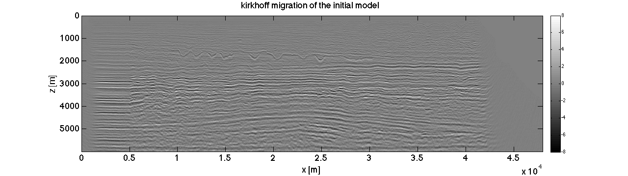
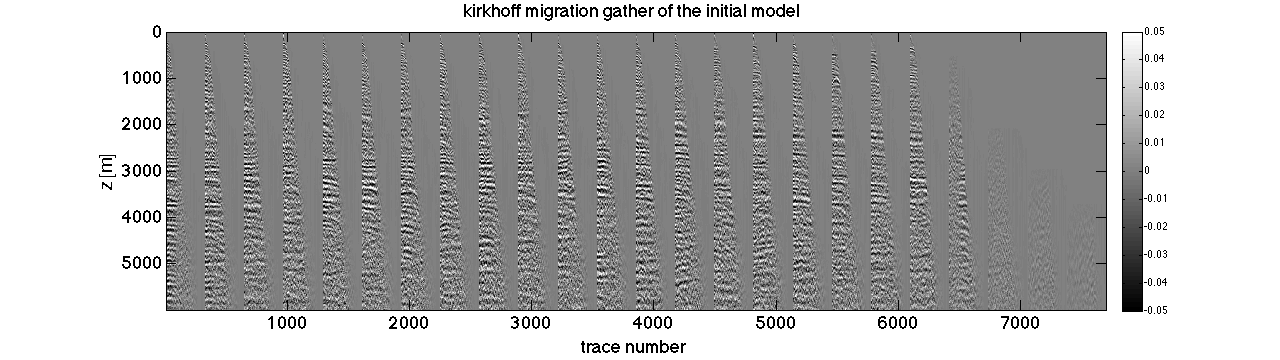
The dataset is very challenging because of the limited offset. According to ray paths in the first figure, turning wave (refraction wave) can not reach the area below 2km, thus the velocity below 2km can not be updated with low-frequency component from turning wave. According to the kirchhoff migration result of the time domain GN FWI result, the moveout corresponding to the area below 2km is not flattened. To address this issue, we scale the velocity below 2km with 0.9 based on the flatness of the moveout roughly.

load model_fwi_mask.mat
scrsz = get(0,'ScreenSize');
figure('Position',[1 scrsz(4)/4 scrsz(3)/2 scrsz(4)/4]);set(gca,'fontsize',18);
imagesc(mmx,mmz,vel_init);caxis([1500,4000]);xlabel('x [m]');ylabel('z [m]');title('scaled initial velocity model[m/s]');colorbar;

load chevron2_reflec_5_nsp_3.mat
scrsz = get(0,'ScreenSize');
figure('Position',[1 scrsz(4)/4 scrsz(3)/2 scrsz(4)/4]);set(gca,'fontsize',18);
imagesc(mmx,mmz,reshape(model.vel, 467,3066));caxis([1500,4000]);xlabel('x [m]');ylabel('z [m]');title('time domain GN FWI with only reflected wave[m/s]');colorbar;

Time domain GN FWI with curvelet domain angle restriction.

As we can observe from the last example, there are a lot of turning artifact in the FWI result. To get rid of those artifacts, we regularize the GN FWI updates in the curvelet domain by setting the curvelet coefficients that corresponding to the vertical events to zeros.

load chevron2_reflec_l1_5_nsp_3.mat
scrsz = get(0,'ScreenSize');
figure('Position',[1 scrsz(4)/4 scrsz(3)/2 scrsz(4)/4]);set(gca,'fontsize',18);
imagesc(mmx,mmz,reshape(model.vel, 467,3066));caxis([1500,4000]);xlabel('x [m]');ylabel('z [m]');title('curvelet-angle restricted time domain GN FWI with only reflected wave[m/s]');colorbar;

load kh_mig.mat
mmx = 0:10:47990;
mmz = 0:10:5990;


scrsz = get(0,'ScreenSize');
figure('Position',[1 scrsz(4)/4 scrsz(3)/2 scrsz(4)/4]);set(gca,'fontsize',18);
imagesc(mmx,mmz,mig_init);caxis(.8e1*[-1 1]);xlabel('x [m]');ylabel('z [m]');colormap gray;title('kirkhoff migration of the initial model');colorbar;
figure('Position',[1 scrsz(4)/4 scrsz(3)/2 scrsz(4)/4]);set(gca,'fontsize',18);
imagesc(mmx,mmz,mig_fwi);caxis(.8e1*[-1 1]);xlabel('x [m]');ylabel('z [m]');colormap gray;title('kirkhoff migration of the final FWI result');colorbar;


figure('Position',[1 scrsz(4)/4 scrsz(3)/2 scrsz(4)/4]);set(gca,'fontsize',18);
imagesc(1:7704,mmz,gather_init);caxis(.5e-1*[-1 1]);xlabel('trace number');ylabel('z [m]');colormap gray;title('kirkhoff migration gather of the initial model');colorbar;
figure('Position',[1 scrsz(4)/4 scrsz(3)/2 scrsz(4)/4]);set(gca,'fontsize',18);
imagesc(1:7704,mmz,gather_fwi);caxis(.5e-1*[-1 1]);xlabel('trace number');ylabel('z [m]');colormap gray;title('kirkhoff migration gather of the final FWI result');colorbar;