Fast Robust Waveform inversion: functions

The functions specific to this package can be found in the mbin directory.

• twonorms - the two-norm and its derivative.
• Jls - least-squares residual and gradient for given model and observed data.
• mylbfgs - standard L-BFGS with Wolfe linesearch

Contents

Penalty functions

The penalty functions are of the form

\(f(\mathbf{r}) = \sum_i p(r_i)\),

where

\(p(r) = \frac{1}{2}r^2\)

for least-squares, which is implemented in the function twonorms. Other penalties can be implemented in a similar fashion.

Misfit functions for FWI

Based on the above penalty functions, we can calculate the misfit for FWI, given a model \(\mathbf{m}\) and observed data \(\mathbf{d}_i\):

\(J(\mathbf{m}) = \sum_i f(F(\mathbf{m})\mathbf{q}_i - \mathbf{d}_i)\),

where \(F(\mathbf{m})\mathbf{q}_i\) is the modeled data for the \(i\)-th source.

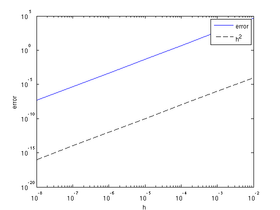
We can test the accuracy of the gradient based on the Taylor series:

\(J(\mathbf{x} + h\Delta \mathbf{x}) = J(\mathbf{x}) + h\nabla J(\mathbf{x})^T\Delta\mathbf{x} + \mathcal(O)(h^2)\)

We can plot the error

\( | J(\mathbf{x}+h\Delta\mathbf{x}) - J(\mathbf{x}) - h\nabla J(\mathbf{x}+h\Delta\mathbf{x})^T\Delta\mathbf{x} | \)

as a function of \(h\) and verify that it decreases as \(h^2\):

% setup some model parameters
model.o = [0 0];
model.d = [10 10];
model.n = [51 51];
model.nb = [50 50];
model.freq = [10];
model.f0 = 10;
model.t0 = 0.01;
model.zsrc = 15;
model.xsrc = 0:100:1000;
model.zrec = 10;
model.xrec = 0:20:1000;

% constant velocity 2000 m/s
v0 = 2000;
m  = 1e6/v0.^2*ones(prod(model.n),1);

% random perturbation
dm = randn(prod(model.n),1);

% define point sources and make data
Q = speye(length(model.xsrc));
D = F(m,Q,model);

% define function-handle for misfit
fh = @(x)Jls(x,Q,D,model);

% test for range of h
h = 10.^[-2:-1:-8];
f0 = fh(m);
for k = 1:length(h)
    [f1, g1] = fh(m + h(k)*dm);
    e(k) = abs(f1 + h(k)*g1'*dm - f0);
end

% plot error
figure;
loglog(h,e,h,h.^2,'k--');
xlabel('h');ylabel('error');
legend('error','h^2');

Alternatively, we can check whether

\(\frac{1}{2}(\nabla J(\mathbf{x}_1 + \nabla J(\mathbf{x}_2))^T(\mathbf{x}_2 - \mathbf{x}_1) = J(\mathbf{x}_2) - J(\mathbf{x_1})\)

for small \( | \mathbf{x}_2 - \mathbf{x}_1 |\).

m1 = m + 1e-3*randn(prod(model.n),1);
m2 = m + 1e-3*randn(prod(model.n),1);

[f1,g1] = fh(m1);
[f2,g2] = fh(m2);

.5*(g1 + g2)'*(m2 - m1)/(f2 - f1)

ans =

    1.0017

Optimization

Included is a standard L-BFGS with a Wolfe linesearch, mylbfgs.m (cf. [1]).

References%

[1] J. Nocedal and S.J. Wright, 1999. Numerical Optimization. Springer.