Modeling

Contents

Source representation

We illustrate how we can represent point-sources by adjoint interpolation.

% grid
xc = [0:1/5:1];
xs = 0.5;

% linear interpolation
P1    = zeros(1,6);
P1(3) = (xs - xc(4))/(xc(3) - xc(4));
P1(4) = (xs - xc(3))/(xc(4) - xc(3));

% quadratic interpolation
P2    = zeros(1,6);

P2(2) = (xs - xc(3))/(xc(2) - xc(3))*(xs - xc(4))/(xc(2) - xc(4));
P2(3) = (xs - xc(2))/(xc(3) - xc(2))*(xs - xc(4))/(xc(3) - xc(4));
P2(4) = (xs - xc(2))/(xc(4) - xc(2))*(xs - xc(3))/(xc(4) - xc(3));

% cubic interpolation
P3    = zeros(1,6);

P3(2) = (xs - xc(3))/(xc(2) - xc(3))*(xs - xc(4))/(xc(2) - xc(4))*(xs - xc(5))/(xc(2) - xc(5));
P3(3) = (xs - xc(2))/(xc(3) - xc(2))*(xs - xc(4))/(xc(3) - xc(4))*(xs - xc(5))/(xc(3) - xc(5));
P3(4) = (xs - xc(2))/(xc(4) - xc(2))*(xs - xc(3))/(xc(4) - xc(3))*(xs - xc(5))/(xc(4) - xc(5));
P3(5) = (xs - xc(2))/(xc(5) - xc(2))*(xs - xc(3))/(xc(5) - xc(3))*(xs - xc(4))/(xc(5) - xc(4));

The resulting discretized delta functions are shown below.

% plot
figure;
plot(xc,P1'*1,xc,P2'*1,xc,P3'*1);legend('linear','quadratic','cubic');
xlabel('x_C');

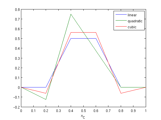
The order up to which the discretized delta function behaves like a true delta function is determined by the order of the interpolation. A table with the error is shown below.

% error
for l = [0:1:5]
    error1(l+1) = abs((xc.^l)*(P1'*1) - xs^l);
    error2(l+1) = abs((xc.^l)*(P2'*1) - xs^l);
    error3(l+1) = abs((xc.^l)*(P3'*1) - xs^l);
end

fprintf(1,'l, linear  , quad.   , cubic\n');
fprintf(1,'%d, %1.2e, %1.2e, %1.2e\n',[[0:5];error1;error2;error3 ]);

l, linear  , quad.   , cubic
0, 0.00e+00, 0.00e+00, 0.00e+00
1, 0.00e+00, 5.55e-17, 5.55e-17
2, 1.00e-02, 0.00e+00, 0.00e+00
3, 1.50e-02, 3.00e-03, 0.00e+00
4, 1.51e-02, 5.10e-03, 9.00e-04
5, 1.27e-02, 5.55e-03, 2.25e-03