Examples
Contents
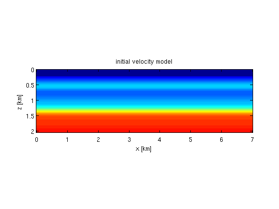
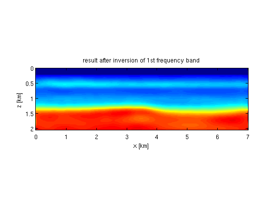
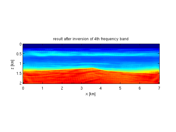
FWI
see example_fwi.m
[v,o,d,n] = odnread(['../data/bg_vp.odn']);
[v0,o,d,n] = odnread(['../data/bg_v0.odn']);

[m1,o,d,n] = odnread(['../results/fwi/m_ls_1.odn']);
[m2,o,d,n] = odnread(['../results/fwi/m_ls_2.odn']);
[m3,o,d,n] = odnread(['../results/fwi/m_ls_3.odn']);
[m4,o,d,n] = odnread(['../results/fwi/m_ls_4.odn']);

[z,x] = odn2grid(o,d*1e-3,n);

figure;
imagesc(x,z,1e-3*reshape(v,n),[1.5 4.5]);
xlabel('x [km]');ylabel('z [km]');axis equal tight;
title('BG Compass velocity model');

figure;
imagesc(x,z,1e-3*reshape(v0,n),[1.5 4.5]);
xlabel('x [km]');ylabel('z [km]');axis equal tight;
title('initial velocity model');

figure;
imagesc(x,z,reshape(real(1./sqrt(m1)),n),[1.5 4.5]);
xlabel('x [km]');ylabel('z [km]');axis equal tight;
title('result after inversion of 1st frequency band');

figure;
imagesc(x,z,reshape(real(1./sqrt(m2)),n),[1.5 4.5]);
xlabel('x [km]');ylabel('z [km]');axis equal tight;
title('result after inversion of 2nd frequency band');

figure;
imagesc(x,z,reshape(real(1./sqrt(m3)),n),[1.5 4.5]);
xlabel('x [km]');ylabel('z [km]');axis equal tight;
title('result after inversion of 3rd frequency band');

figure;
imagesc(x,z,reshape(real(1./sqrt(m4)),n),[1.5 4.5]);
xlabel('x [km]');ylabel('z [km]');axis equal tight;
title('result after inversion of 4th frequency band');


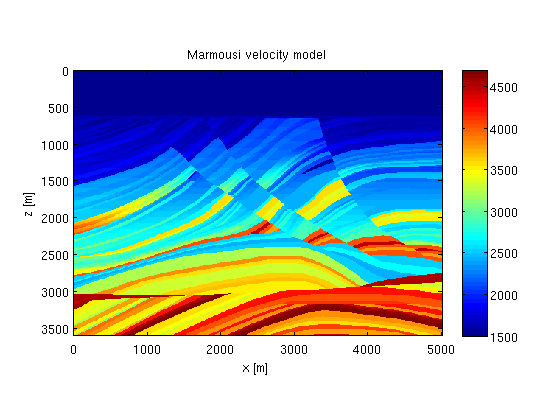
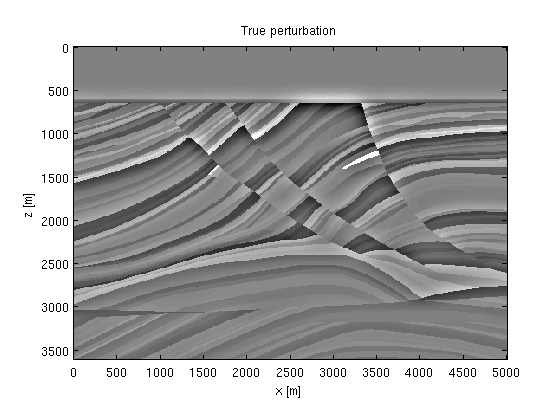
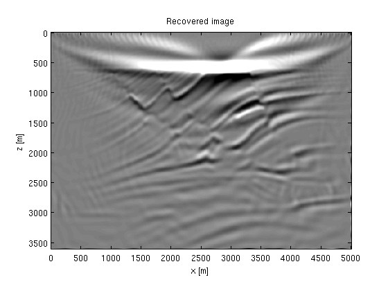
Reverse time migration
see example_rtm.m
[v,o,d,n]  = odnread(['../data/marm_vp.odn']);
v = reshape(v,n);
v = [1500*ones(60,501); v(1:301,500 + [1:501])];
n = size(v);
S = opKron(opSmooth(n(2),200),opSmooth(n(1),200));

% smooth model
m  = 1e6./v(:).^2;
m0 = S*m;
dm = m - m0;
dm = reshape(dm,n);
v0 = reshape(1e3./sqrt(m0),n);
[dmt,o,d,n] = odnread(['../results/rtm/dmt.odn']);dmt=reshape(dmt,n);

[z,x] = odn2grid(o,d,n);

figure;
imagesc(x,z,v,[1500 4700]);colorbar;
xlabel('x [m]');ylabel('z [m]');
axis equal tight;
title('Marmousi velocity model')

figure;
imagesc(x,z,v0,[1500 4700]);colorbar;
xlabel('x [m]');ylabel('z [m]');
axis equal tight;
title('Reference velocity used for RTM')

figure;
imagesc(x,z,dm,[-1 1]*1e-1);colormap(gray);
xlabel('x [m]');ylabel('z [m]');
axis equal tight;
title('True perturbation');

figure;
imagesc(x,z,dmt,[-1 1]*1e6);colormap(gray);
xlabel('x [m]');ylabel('z [m]');
axis equal tight;
title('Recovered image');

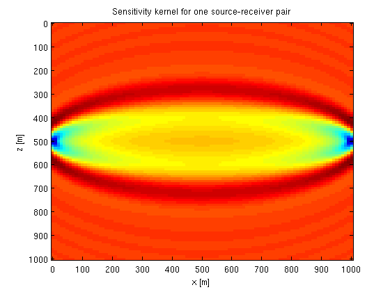
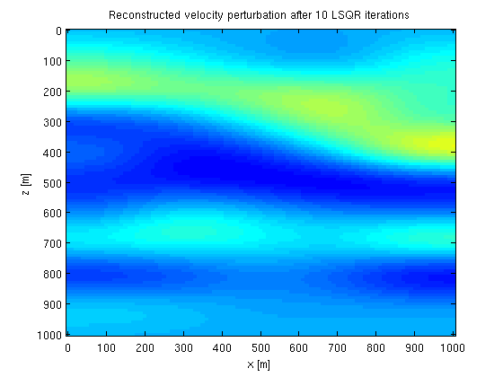
Traveltime tomography
see example_tomo.m
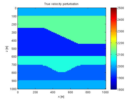
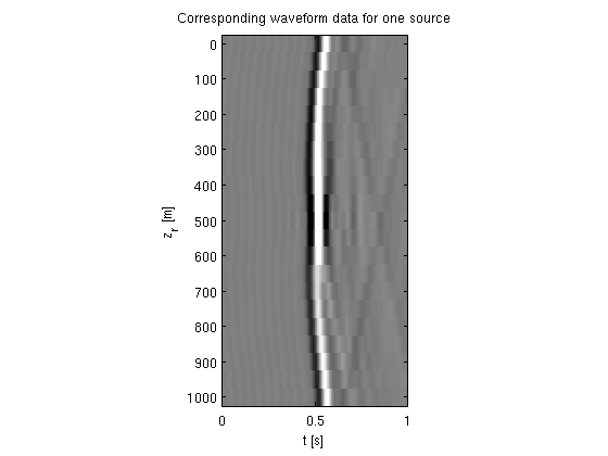
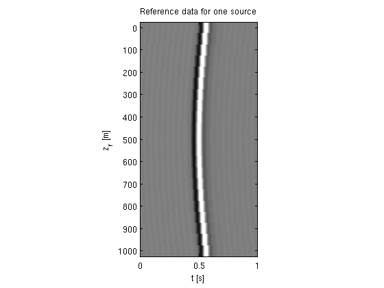
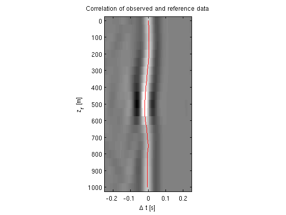
[Dt,od,dd,nd] = odnread(['../results/tomo/Dt.odn']);
Dt = reshape(Dt,nd);
[D0t,od,dd,nd] = odnread(['../results/tomo/D0t.odn']);
D0t = reshape(D0t,nd);
[Ct,od,dd,nd] = odnread(['../results/tomo/Ct.odn']);
Ct = reshape(Ct,nd);

T = odnread(['../results/tomo/croswell_time.odn']);
T = reshape(T,nd(1:2));

[k1,o,d,n] = odnread(['../results/tomo/k1.odn']);
k1 = reshape(k1,n);

[dm,o,d,n] = odnread(['../data/crosswell_vp.odn']);
dm = reshape(dm,n);

[dmt,o,d,n] = odnread(['../results/tomo/dmt.odn']);
dmt = reshape(dmt,n);

[zrec,zsrc,t] = odn2grid(od,dd,nd);
[z,x] = odn2grid(o,d,n);

figure;
imagesc(x,z,dm,[1800 2500]);
xlabel('x [m]');ylabel('z [m]');colorbar;
title('True velocity perturbation')

figure;
imagesc(t,zrec,-squeeze(Dt(:,11,:)),[-1 1]*2e2);colormap(gray);
ylabel('z_r [m]');xlabel('t [s]');xlim([0 1]);
set(gca,'plotboxaspectratio',[1 2 1]);
title('Corresponding waveform data for one source')

figure;
imagesc(t,zrec,-squeeze(D0t(:,11,:)),[-1 1]*2e2);colormap(gray);
ylabel('z_r [m]');xlabel('t [s]');xlim([0 1]);
set(gca,'plotboxaspectratio',[1 2 1]);
title('Reference data for one source')

figure;
imagesc(t-1,zrec,fftshift(squeeze(Ct(:,11,:)),2),[-1 1]*4e4);colormap(gray);
ylabel('z_r [m]');xlabel('\Delta t [s]');xlim([-.25 .25]);set(gca,'plotboxaspectratio',[1 2 1]);
tmp=fftshift(squeeze(Ct(:,11,:)),2);
[~,it] = max(tmp,[],2);
hold on;plot(t(it)-1,zrec,'r')
title('Correlation of observed and reference data')

figure;
imagesc(zrec,zsrc,T);
xlabel('z_r [m]');ylabel('z_s [m]');colorbar
title('Traveltime data for each source/receiver pair');

figure;
imagesc(x,z,k1);
xlabel('x [m]');ylabel('z [m]');
title('Sensitivity kernel for one source-receiver pair')

figure;
imagesc(x,z,1e3./sqrt(.25+dmt),[1800 2500]);
xlabel('x [m]');ylabel('z [m]');
title('Reconstructed velocity perturbation after 10 LSQR iterations')