2D time-domain acoustic anisotropic and acoustic isotropic modelling and linearized modelling demo

The modeling operator is based on a star 1D stencil of order 2,4 or 6. It solves the system in parallel over sources . Source injection and receiver sampling is done via cubic interpolation and exponential damping over a 3x3 square around the source location. The Jacobian is derived by linearizing the discretized system and its forward and adjoint action is calculated via the adjoint-state method.

The basic syntax of the modeling operator is data = Gen_data(m,Q,model,density,anisotropy)|, where

• m is a vector with a gridded slowness-squared model [km^2/s^2],
• Q is a vectorof that defines the source,
• model is a struct with various other parameters,
• data is a vectorized data-cube (receiver x source x time),
• density is the density
• anisotropy are the thompsen parameters

We illustrate the basic modeling capabilities on a simple layered model.

Contents

medium parameters

o = [0, 0]; % Origin
n = [162, 600]; % Size of the domain in grid points
N = prod(n);
d = [15, 15]; % Grid size of the original model
v = ones(n)*1.400;
% velocity [km/s]
v(50:100,:) = 2.000;
v(101:end,:) = 3.000;
v = v(:);
m=1./v.^2; % square slowness
% Thompsen parameters
ani.delta = ones(N,1)*0.3;
ani.epsilon = ones(N,1)*0.2;
ani.theta = ones(N,1)*pi/9;

Model containing acquisition geometry and modelling parameters

model.o=[o 0]; %Origins of the axes [m]
model.n=[n 1]; %Number of grid points  for each dimension (excluding boundaries)
model.d=[d d(1)];
model.ddcompx=1; % Domain decomposition x direction
model.ddcompy=1; % Domain decomposition y direction
model.ddcompz=1; % Domain decomposition z direction
model.f0=0.015; % in [kHz]
model.xsrc =4500; % Source position along x axis in [m]
model.zsrc= 10*ones(size(model.xsrc)); %Source coordinates along z axis [m]
model.ysrc=0*ones(size(model.xsrc));%Source coordinates along y axis [m] (still necessary for 2D will be removed)
model.xrec = 0:15:9000;%Receivers coordinates along x axis [m]
model.zrec=10; %Receivers coordinates along z axis [m]
model.yrec=0; %Receivers coordinates along y axis [m]
model.T=2000; %Acquisition duration [ms]
model.freesurface=0; % Freesurface ( 0 : no freesurface, 1 : freesurface)
model.space_order=2; % Space discretization order (2,4 or 6 only for now)
model.type='full'; % Type of aquisition : 'marine' or 'full' (split-pread)
model.gppwl = 7;    % grid points per wave length (only for anisotropy)

Acoustic isotropic modeling

[m1,model1]=Setup_CFL(m,model); % Setup dt, new grid size and new model for given peak frequency
model1.NyqT=0:4:model1.T; % Shot record time axis
q=sp_RickerWavelet(model1.f0,1/model1.f0,model1.dt,model1.T); % Source

tic;
dataT1=Gen_data(m1,model1,q); % Generate data, can also be called with Gen_data(m2,model2,q,[],[])
toc

CFL conditions gives dt = 1.9092ms and d = 9  9  9 m 
Velocity interpolated on new grid
shot = 4500
Acoustic isotropic
Elapsed time is 9.217471 seconds.

Acoustic anisotropic modeling

[m2,model2,~,ani2]=Setup_CFL(m,model,[],ani);% Setup dt, new grid size and new model for given peak frequency
model2.NyqT=0:4:model2.T;% Shot record time axis
q=sp_RickerWavelet(model2.f0,1/model2.f0,model2.dt,model2.T);% sources

tic;
dataT2=Gen_data(m2,model2,q,[],ani2);
toc

CFL conditions gives dt = 1.7556ms and d = 13  13  13 m 
Velocity interpolated on new grid
shot = 4500
Acoustic anisotropic
Elapsed time is 41.756172 seconds.

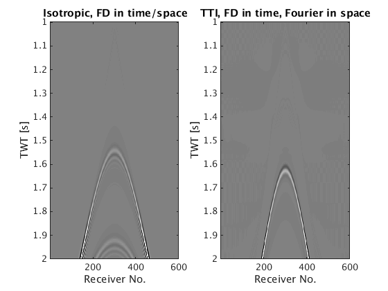
Reshape and display results

dataT1=reshape(dataT1,length(model1.NyqT),length(model1.xrec)*length(model1.zrec)*length(model1.yrec),length(model1.xsrc));
rec = 1:length(model1.xrec); tt = 1:model1.T/1000;
figure(1);subplot(1,2,1); imagesc(rec,tt,dataT1); caxis([-10 10]);colormap(gray);
title('Isotropic, FD in time/space'); xlabel('Receiver No.'); ylabel('TWT [s]')

dataT2=reshape(dataT2,length(model2.NyqT),length(model2.xrec)*length(model2.zrec)*length(model2.yrec),length(model2.xsrc));
subplot(1,2,2); imagesc(rec,tt,dataT2); caxis([-10 10]);colormap(gray);
title('TTI, FD in time, Fourier in space'); xlabel('Receiver No.'); ylabel('TWT [s]')

Born modelling

The basic syntax of the Born modeling operator is du = Born(m,Q,model,din,mode,density,anisotropy)|, A more detailed documentation of the function will be added in a Time imaging section where

Smooth model

S  = opKron(opSmooth(n(2),100),opSmooth(n(1),200));  %smoothing operator
v0=S*v(:);
m0=1./v0.^2;
% Model perturbations
dm=m-m0;

Linearized acoustic isotropic

You need to put dm in the Setup_CFL to project it on the new grid as well

[m1,model1,dm1]=Setup_CFL(m0,model,dm);
model1.NyqT=0:4:model1.T;
q=sp_RickerWavelet(model1.f0,1/model1.f0,model1.dt,model1.T);
du1=Born(m1,model1,q,dm1,1);

CFL conditions gives dt = 1.9092ms and d = 9  9  9 m 
Velocity interpolated on new grid
J for shot  1 over 1 at position 4500
Acoustic isotropic

Linearized acoustic anisotropic

[m2,model2,dm2,ani2]=Setup_CFL(m0,model,dm,ani);
model2.NyqT=0:4:model2.T;
q=sp_RickerWavelet(model2.f0,1/model2.f0,model2.dt,model2.T);
du2=Born(m2,model2,q,dm2,1,[],ani2);

CFL conditions gives dt = 1.7556ms and d = 13  13  13 m 
Velocity interpolated on new grid
J for shot  1 over 1 at position 4500
Acoustic anisotropic

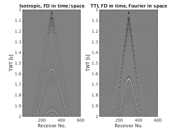
Reshape and display results

du1=reshape(du1,length(model1.NyqT),length(model1.xrec)*length(model1.zrec)*length(model1.yrec),length(model1.xsrc));
rec = 1:length(model1.xrec); tt = 1:model1.T/1000;
figure(2);subplot(1,2,1); imagesc(rec,tt,du1); caxis([-10 10]);colormap(gray);
title('Isotropic, FD in time/space'); xlabel('Receiver No.'); ylabel('TWT [s]')

du2=reshape(du2,length(model2.NyqT),length(model2.xrec)*length(model2.zrec)*length(model2.yrec),length(model2.xsrc));
subplot(1,2,2); imagesc(rec,tt,du2); caxis([-10 10]);colormap(gray);
title('TTI, FD in time, Fourier in space'); xlabel('Receiver No.'); ylabel('TWT [s]')