2D time-stepping modeling
Author: Dr. Xiang Li
       Seismic Laboratory for Imaging and Modeling
       Department of Earch & Ocean Sciences
       The University of British Columbia
Date: July, 2015
This is an demo script of the SLIM version time-steppling modeling kernel You can find the modeling code SLIM software release under tools/algorithms/TimeModeling.
Contents
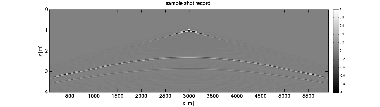
demo of generation a shot record.
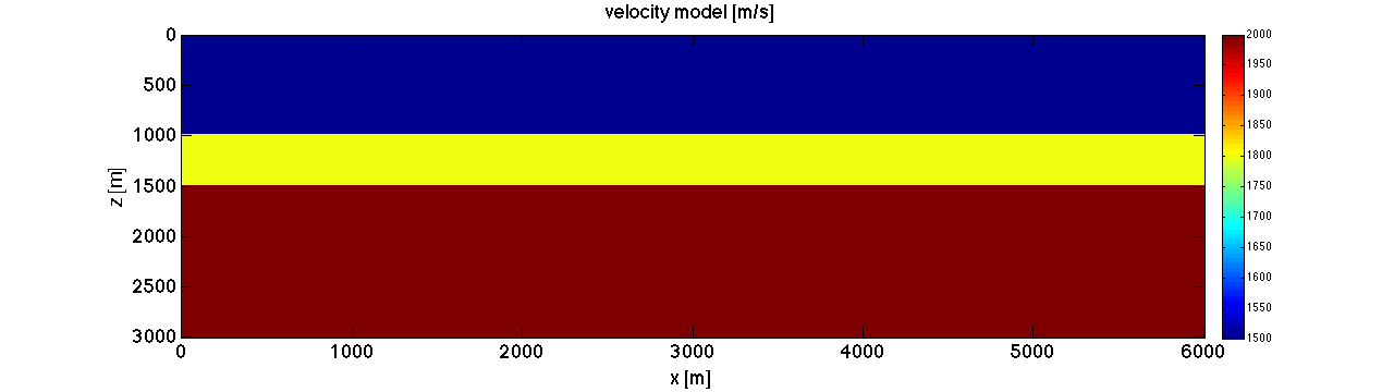
velocity model. please do 'help XiangLi_Time' for the meanning of different paras
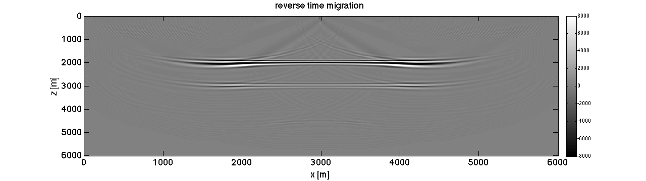
mmx = linspace(0,6000,601);
mmz = linspace(0,3000,301);
mmy = 1;

nz = length(mmz);
nx = length(mmx);
ny = length(mmy);

vel = 1500 * ones(nz,nx,ny);
vel(100:end,:) = 1800;
vel(150:end,:) = 2000;
% initial model
Ps = opSmooth(nz,50);

scrsz = get(0,'ScreenSize');
figure('Position',[1 scrsz(4)/4 scrsz(3)/2 scrsz(4)/4]);set(gca,'fontsize',18);
imagesc(mmx,mmz,vel);xlabel('x [m]');ylabel('z [m]');title('velocity model [m/s]');colorbar;

vel_init = Ps * vel;
den = ones(size(vel));
% den(300:end,:) = 2;

vel 	 = vel(:);
vel_init = vel_init(:);
dv		 = 1./vel - 1./vel_init;
den		 = den(:);
% den = .23 * vel.^.25;


model.vel = vel;
model.den = den;


model_init.vel = vel_init;
model_init.den = den;

% set source location and receiver location
fwdpara.stype = 'seq_same';

fwdpara.slz   = [ mmz(2) ];
fwdpara.slx   = [ mmx(300) ];
fwdpara.sly   = [1];


fwdpara.saved = 1;
fwdpara.shot_id = 1;
dr  = 5;
rlx = mmx(10:5:end-10);
% rlx = fwdpara.slx:10:fwdpara.slx+1000;
rly = 1;
rlz = mmz(2);

[rlx,rlz,rly] = meshgrid(rlx,rlz,rly);

fwdpara.rtype = 'marine';
fwdpara.rlx = [rlx(:)];
fwdpara.rlz = [rlz(:)];
fwdpara.rly = [rly(:)];


% source wavelet
fwdpara.fcent = 15;
fwdpara.dt    = .003;
t     = 4;
t0    = 1;
[src,fwdpara.taxis] = wvlet2(fwdpara.fcent,fwdpara.dt,t,t0);

% size of PML boundary in terms of model grids.
fwdpara.abx = 40;
fwdpara.abz = 40;
fwdpara.aby = 40;

fwdpara.free = 1;


% domain decomposition,
%
% BE SURE number of workers =  fwdpara.ddcompx X fwdpara.ddcompz X fwdpara.ddcompy
%
%
fwdpara.ddcompx = 1;
fwdpara.ddcompz = 1;
fwdpara.ddcompy = 1;

fwdpara.mmx = mmx;
fwdpara.mmz = mmz;
fwdpara.mmy = mmy;

% optimal checkpoints, do "help  XiangLi_Time"
fwdpara.chkp_space	= 50;
fwdpara.chkp_save	= 2;


fwdpara.disp_snapshot = 0;% set to "1" if you want so see the snapshot. ONLY WORK WHEN YOU USE ONE WORKER.
fwdpara.wave_equ = 1;
fwdpara.v_up_type = 'slowness';
fwdpara.space_order = 4;

% do forward modeling with true model.
fwdpara.fmode = 1;
[Ur] = XiangLi_Time(model,src,fwdpara);


U_obs_shot_record = reshape(gather(Ur),length(fwdpara.taxis),length(fwdpara.rlx));
scrsz = get(0,'ScreenSize');
figure('Position',[1 scrsz(4)/4 scrsz(3)/2 scrsz(4)/4]);set(gca,'fontsize',18);
imagesc(fwdpara.rlx,fwdpara.taxis,U_obs_shot_record);caxis([-1,1]);xlabel('x [m]');ylabel('z [m]');
title('sample shot record');colorbar;colormap gray


% do forward modeling with initial model
[Ur1,chk] = XiangLi_Time(model_init,src,fwdpara);

dUr = Ur - Ur1;
%
Ps = op_XiangLi_Time(model_init,src,fwdpara,chk);

g = Ps' * dUr;

g =  reshape(g,length(fwdpara.mmz),length(fwdpara.mmx));

scrsz = get(0,'ScreenSize');
figure('Position',[1 scrsz(4)/4 scrsz(3)/2 scrsz(4)/4]);set(gca,'fontsize',18);
imagesc(fwdpara.mmx,fwdpara.mmx,g);caxis(1e3*[-8,8]);xlabel('x [m]');ylabel('z [m]');
title('reverse time migration');colormap gray;colorbar
--------------------------------------------------------------------------------
          Solving forward modeling from T1 to Tmax
--------------------------------------------------------------------------------
     ----- Simulating shot 1 -----
          Time=0.147s, Total=3.999s.
          Time=0.297s, Total=3.999s.
          Time=0.447s, Total=3.999s.
          Time=0.597s, Total=3.999s.
          Time=0.747s, Total=3.999s.
          Time=0.897s, Total=3.999s.
          Time=1.047s, Total=3.999s.
          Time=1.197s, Total=3.999s.
          Time=1.347s, Total=3.999s.
          Time=1.497s, Total=3.999s.
          Time=1.647s, Total=3.999s.
          Time=1.797s, Total=3.999s.
          Time=1.947s, Total=3.999s.
          Time=2.097s, Total=3.999s.
          Time=2.247s, Total=3.999s.
          Time=2.397s, Total=3.999s.
          Time=2.547s, Total=3.999s.
          Time=2.697s, Total=3.999s.
          Time=2.847s, Total=3.999s.
          Time=2.997s, Total=3.999s.
          Time=3.147s, Total=3.999s.
          Time=3.297s, Total=3.999s.
          Time=3.447s, Total=3.999s.
          Time=3.597s, Total=3.999s.
          Time=3.747s, Total=3.999s.
          Time=3.897s, Total=3.999s.
--------------------------------------------------------------------------------
  Max space interval is 10m, which is larger than optinal 10m.
  Modify it to optinal or lower the centrel frequency of your wavelet to 15Hz
--------------------------------------------------------------------------------
--------------------------------------------------------------------------------
          Solving forward modeling from T1 to Tmax
--------------------------------------------------------------------------------
     ----- Simulating shot 1 -----
          Time=0.147s, Total=3.999s.
          Time=0.297s, Total=3.999s.
          Time=0.447s, Total=3.999s.
          Time=0.597s, Total=3.999s.
          Time=0.747s, Total=3.999s.
          Time=0.897s, Total=3.999s.
          Time=1.047s, Total=3.999s.
          Time=1.197s, Total=3.999s.
          Time=1.347s, Total=3.999s.
          Time=1.497s, Total=3.999s.
          Time=1.647s, Total=3.999s.
          Time=1.797s, Total=3.999s.
          Time=1.947s, Total=3.999s.
          Time=2.097s, Total=3.999s.
          Time=2.247s, Total=3.999s.
          Time=2.397s, Total=3.999s.
          Time=2.547s, Total=3.999s.
          Time=2.697s, Total=3.999s.
          Time=2.847s, Total=3.999s.
          Time=2.997s, Total=3.999s.
          Time=3.147s, Total=3.999s.
          Time=3.297s, Total=3.999s.
          Time=3.447s, Total=3.999s.
          Time=3.597s, Total=3.999s.
          Time=3.747s, Total=3.999s.
          Time=3.897s, Total=3.999s.
Warning: Data type "distributed" is not officially supported by spot, proceed
at own risk
--------------------------------------------------------------------------------
  Max space interval is 10m, which is larger than optinal 10m.
  Modify it to optinal or lower the centrel frequency of your wavelet to 15Hz
--------------------------------------------------------------------------------
--------------------------------------------------------------------------------
          Gradient of FWI objective function.
--------------------------------------------------------------------------------
     ----- Simulating shot 1 -----
          Time=3.897s, Total=3.999s.
          Time=3.747s, Total=3.999s.
          Time=3.597s, Total=3.999s.
          Time=3.447s, Total=3.999s.
          Time=3.297s, Total=3.999s.
          Time=3.147s, Total=3.999s.
          Time=2.997s, Total=3.999s.
          Time=2.847s, Total=3.999s.
          Time=2.697s, Total=3.999s.
          Time=2.547s, Total=3.999s.
          Time=2.397s, Total=3.999s.
          Time=2.247s, Total=3.999s.
          Time=2.097s, Total=3.999s.
          Time=1.947s, Total=3.999s.
          Time=1.797s, Total=3.999s.
          Time=1.647s, Total=3.999s.
          Time=1.497s, Total=3.999s.
          Time=1.347s, Total=3.999s.
          Time=1.197s, Total=3.999s.
          Time=1.047s, Total=3.999s.
          Time=0.897s, Total=3.999s.
          Time=0.747s, Total=3.999s.
          Time=0.597s, Total=3.999s.
          Time=0.447s, Total=3.999s.
          Time=0.297s, Total=3.999s.
          Time=0.147s, Total=3.999s.
Jacobian test.
all the following test can be reproduced with the scipt 'demo2D_gradient_test.m'
- linear modeling operater test
F(m+dm) = F[m0] + J * dm + o{||dm||_2};
F is modeling function 'XiangLi_Time'. J is the adjoint of migration operator
J and J' can be generated with 'op_XiangLi_Time';
Testing result is shown in Figure demo2d_gradient.png
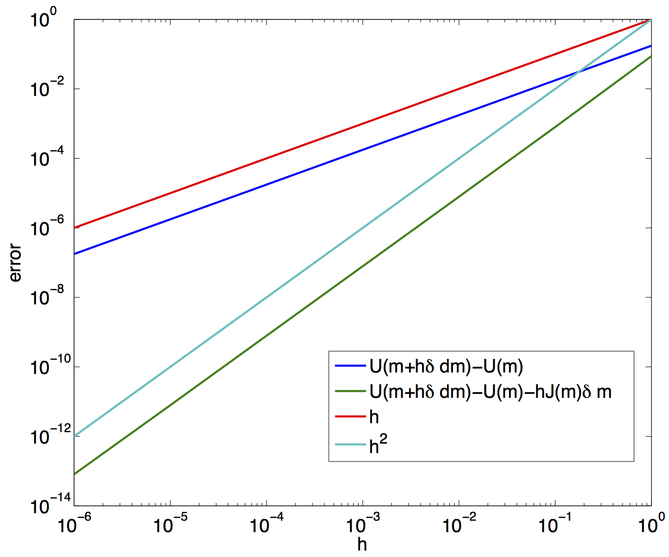
- gradient test of Jocaobian.
consider the taylor expension of FWI objective function
\phi(m) = \frac{1}{2}\|F(m)-D\|_2
\phi{m+h*dm} = \phi{m} + h * J' * dm + o{h^2}
Testing result is shown in Figure demo2d_gradient_fwiobj.png
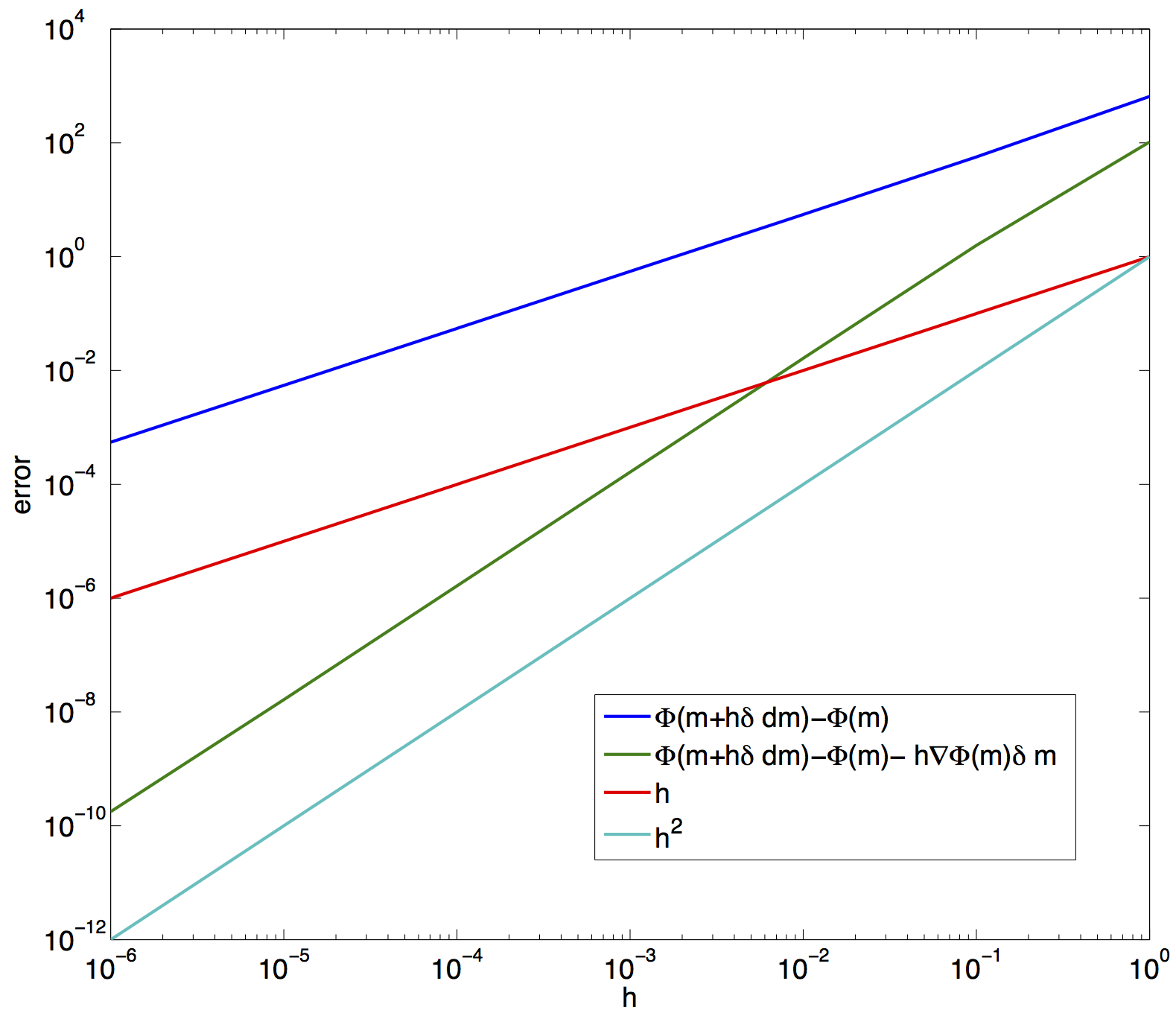