2D constant-density acoustic frequency-domain modeling, linearized modeling and imaging: Testing

This script presents some basic tests of the modeling code.

Analytic solution for constant medium
Analytic solution for linear velocity profile
Jacobian test
Adjoint test
References

Analytic solution for constant medium

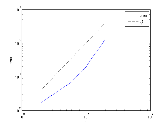
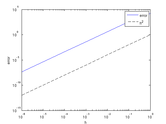
We test the code against the analytic solution for a constant velocity and plot the error as a function of the gridspacing to verify the order of accuracy of the discretization. The 9-point mixed-grid discretization of [1] uses a regular and rotated 5-point discretization of the Laplace operator, which makes it technically a second-order scheme. It is optimized to minimize numerical dispersion, though, and hence expected to be more accurate than a regular 5-point discretization.

% velocity [m/s]
v0 = 2000;

% size of domain LxL m
L = 1000;

% sponge boundary size B m
B = 250;

% frequency [1/s]
f  = 10;

% gridspacings
h = [20:-2:2];
e = 0*h;
% loop
for k = 1:length(h)
    % grid paramets
    model.o = [0 0];
    model.d = [h(k) h(k)];
    model.n = [floor(L/h(k)) + 1 floor(L/h(k)) + 1];

    % source and receiver setup
    model.zsrc = 500;
    model.xsrc = 500;
    model.zrec = 0:h(k):L;
    model.xrec = 0:h(k):L;

    % absorbing boundary
    model.nb = [floor(B/h(k)) + 1 floor(B/h(k))];

    % frequency
    model.freq = f;

    % ricker wavelet
    model.f0 = 0;
    model.t0 = 0;

    % source matrix
    Q = 1;

    % slowness-squares model [km^2/s^2]
    m  = 1e6*ones(prod(model.n),1)./v0.^2;

    % analytic solution
    D1 = G([v0;0],Q,model);

    % numerical solution
    D2 = F(m,Q,model,1);

    % error
    e(k) = norm(D1 - D2);
end

The figure below confirms that the scheme is second order.

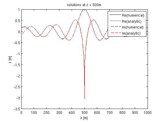
% plot error
figure;
loglog(h,e,h,h.^2,'k--');
xlabel('h');ylabel('error');legend('error','h^2');

% plot
z = 0:h(k):1000;
x = 0:h(k):1000;
D1 = reshape(D1,model.n);
D2 = reshape(D2,model.n);

iz = floor(length(z)/2) + 1;

figure;
plot(x,real(D1(iz,:)),'k',x,real(D2(iz,:)),'r',x,imag(D1(iz,:)),'k--',x,imag(D2(iz,:)),'r--');
legend('Re(numerical)','Re(analytic)','Im(numerical)','Im(analytic)');
xlabel('x [m]');ylabel('z [m]');
title(['solutions at z = ' num2str(z(iz)) 'm']);

Analytic solution for linear velocity profile

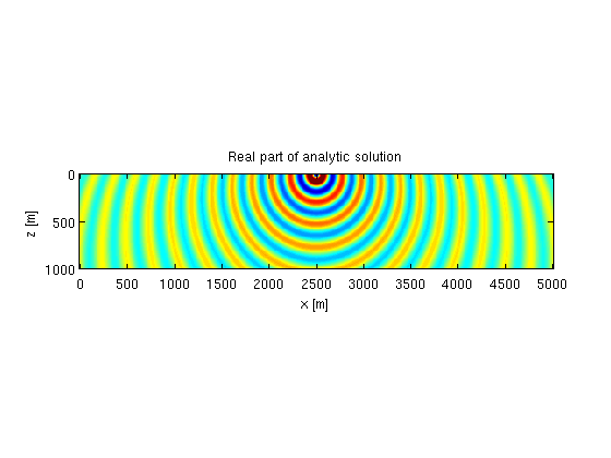
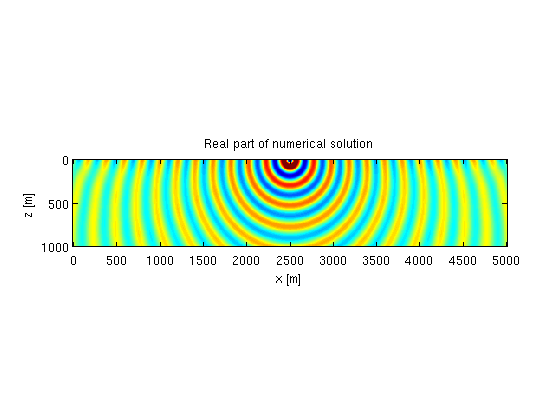
The analytic Greens function for a linear velocity profile \(v = v_0 + \alpha z\) is presented by [2]. An example is shown below.

% velocity profile
v0 = 2000;
alpha = 0.7;

% grid
z = 0:10:1000;
x = 0:10:5000;
[o,d,n] = grid2odn(z,x);

% gridded slowness-squared
m = vec((1e6./(v0+alpha*z').^2)*ones(size(x)));

% frequency
f = 10;

% modeling parameters
model.o = o;
model.d = d;
model.n = n;
model.nb = [50 50];
model.freq = f;
model.f0 = 0;
model.t0 = 0;
model.zsrc = 10;
model.xsrc = mean(x);
model.zrec = z;
model.xrec = x;

% source
Q = 1;

% analytic solution
G1 = G([v0;alpha],Q,model);

% numerical solution
G2 = F(m,Q,model,1);

% plot
figure;
imagesc(x,z,reshape(real(G1),n),[-10 10]);axis equal tight;
title('Real part of analytic solution');
xlabel('x [m]');ylabel('z [m]');

figure;
imagesc(x,z,reshape(real(G2),n),[-10 10]);axis equal tight;
title('Real part of numerical solution');
xlabel('x [m]');ylabel('z [m]');

Jacobian test

The Jacobian of the modeling operator is derived by linearizing the discretized system. We can test the accuracy by considering the Taylor approximation

\(F(\mathbf{m} + h\delta\mathbf{m}) = F(\mathbf{m}) + hJ\delta\mathbf{m} + \mathcal{O}(h^2).\)

% setup model parameters
model.o = [0 0];
model.d = [10 10];
model.n = [101 101];
model.nb = [20 20];
model.freq = [10 15];
model.f0 = 10;
model.t0 = 0.01;
model.zsrc = 15;
model.xsrc = 0:100:1000;
model.zrec = 10;
model.xrec = 0:5:1000;

% source matrix
Q = speye(length(model.xsrc));

% constant velocicty
v0 = 2000;
m  = 1e6/v0.^2*ones(prod(model.n),1);

% random perturbation, set values close to the edge to zero.
dm = randn(model.n);
dm([1:20 end-20:end],:) = 0;
dm(:,[1:20 end-20:end]) = 0;
dm = dm(:);

% data and Jacobian
[D0, J0] = F(m,Q,model);

% linearized data
dD = J0*dm;

% stepsizes
h = 10.^[0:-1:-6];
e = 0*h;

for k = 1:length(h)
    D1   = F(m+h(k)*dm,Q,model);
    e(k) = norm(D1 - D0 - h(k)*dD);
end

% plot error
figure;
loglog(h,e,h,h.^2,'k--');
xlabel('h');ylabel('error');legend('error','h^2');

The figure confirms the error decreases as \(h^2\).

Adjoint test

The adjoint test will ensure that our implementation of the adjoint satisfies the formal definition of the adjoint:

\(\langle A\mathbf{x},\mathbf{y}\rangle = \langle \mathbf{x},A^*\mathbf{y}\rangle\)

% setup model parameters
model.o = [0 0];
model.d = [10 10];
model.n = [51 51];
model.nb = [10 10];
model.freq = [10 15];
model.f0 = 10;
model.t0 = 0.01;
model.zsrc = 15;
model.xsrc = 0:100:1000;
model.zrec = 10;
model.xrec = 0:5:1000;

% source matrix
Q = speye(length(model.xsrc));

% constant velocicty
v0 = 2000;
m  = 1e6/v0.^2*ones(prod(model.n),1);

% Jacobian operator
J = oppDF(m,Q,model);


% test for 10 random vectors
for k = 1:10
    x = randn(prod(model.n),1);
    y = J*x;

    left(k)  = gather((J*x)'*y);
    right(k) = gather(x'*(J'*y));
end

The quantities left and right should be the same up to numerical precision, which we can easily verify by looking at the relative error:

% error
abs(left - right)./max(abs(left),abs(right))

ans =

   1.0e-15 *

  Columns 1 through 7

    0.1689    0.1655         0         0         0    0.2010    0.1802

  Columns 8 through 10

    0.1255    0.5508    0.1557

References

[1] C-H Jo,* C. Shin,* and J.H. Suh, 1996. An optimal 9-point, finite-difference, frequency-space, 2-D scalar wave extrapolator Geophysics 61(2), 529-537.

[2] B.N. Kuvshinov, W.A. Mulder. The exact solution of the time-harmonic wave equation for a linear velocity profile Geophysical Journal International 167(2), 659–662, 2006.