2D constant-density acoustic frequency-domain modeling, linearized modeling and imaging: Modeling

The modeling operator is based on a 9-point mixed-grid discretization of the Helmholtz operator [1]. It solves the system in parallel over frequencies using direct factorization (Matlab's mldivide). Source injection and receiver sampling is done via cubic interpolation. The Jacobian is derived by linearizing the discretized system and its forward and adjoint action is calculated via the adjoint-state method.

The basic syntax of the modeling operator is [D,J] = F(m,Q,model), where

• m is a vector with a gridded slowness-squared model [km^2/s^2],
• Q is a matrix that defines the sources,
• model is a struct with various other parameters,
• D is a vectorized data-cube (receiver x source x frequency),
• J is the Jacobian as SPOT operator.

We illustrate the basic modeling capabilities on a simple layered model.

Contents

Model

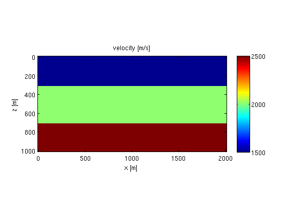
We define a simple layered model:

% grid
z = 0:20:1000;
x = 0:20:2000;

% convert to [origin, increment, size] triplet
[o,d,n] = grid2odn(z,x);

% velocity
v = 1500*ones(n);
v(z>300,:) = 2000;
v(z>700,:) = 2500;

% plot
figure;
imagesc(x,z,v);axis equal tight;colorbar;
xlabel('x [m]');ylabel('z [m]');title('velocity [m/s]');

Now, we define a vector with gridded slowness-squared values [km^2/s^2]

m = 1e6./v(:).^2;

Sources/receivers

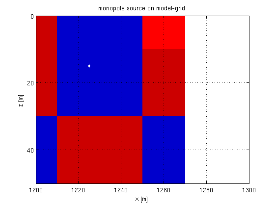
The sources are defined on a separate grid, which is mapped to the computational grid via adjoint cubic interpolation. A monopole source is then simply defined by putting a single spike on the source grid. For example,

% source grid, 1D grid at z = 15
zsrc = 15;
xsrc = 500:25:1500;

% point source at z = 15, x = 1225
q = 0*xsrc;
q(xsrc==1225) = 1;

% define cubic interpolation operator that maps from the model-grid to the
% source-grid:

L = opKron(opLInterp1D(x,xsrc),opLInterp1D(z,zsrc));

% plot source function on model grid
figure;
imagesc(x,z,reshape(L'*q(:),n),[-0.01 0.01]);xlim([1200 1300]);ylim([0 50]);
colormap([.8 0 0;1 0 0;1 1 1;0 0 1;0 0 .8]);
set(gca,'xtick',x,'ytick',z,'xgrid','on','ygrid','on');
hold on;plot(1225,15,'w*');
xlabel('x [m]');ylabel('z [m]');title('monopole source on model-grid');

Each column of the source matrix Q defines one gridded source function. To define a point source on each gridpoint of the source grid, we simply take Q to be an identity matrix:

Q = speye(length(xsrc));

The receivers are defined on a similar grid, and the data is mapped to this grid via cubic interpolation.

Parameters

The struct model contains the following parameters

% model grid
model.o = o;
model.d = d;
model.n = n;

% absorbing boundary
model.nb = [50 50];

% source/receiver grid
model.zsrc = zsrc;
model.xsrc = xsrc;
model.zrec = 5;
model.xrec = 0:15:2000;

% frequencies in Herz.
model.freq = [4:2:15];

% wavelet
model.f0 = 10;
model.t0 = 0.01;

Data

Having defined al the parameters, we can simply generate data as follows

D = F(m,Q,model,1);

The number of source, receivers and frequencies are given by

nrec  = length(model.xrec);
nsrc  = size(Q,2);
nfreq = length(model.freq);

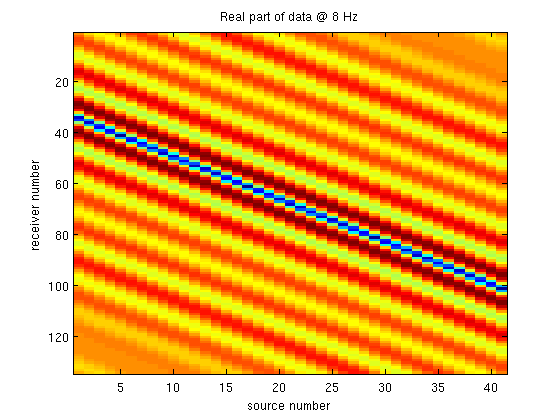
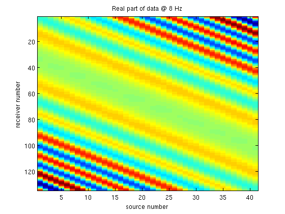
We can now reshape the data into a cube and plot a frequency slice

D = reshape(D,nrec,nsrc,nfreq);

figure;
imagesc(real(D(:,:,3)));
xlabel('source number');ylabel('receiver number');title(['Real part of data @ ' num2str(model.freq(3)) ' Hz']);

Born modeling

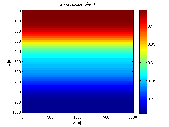
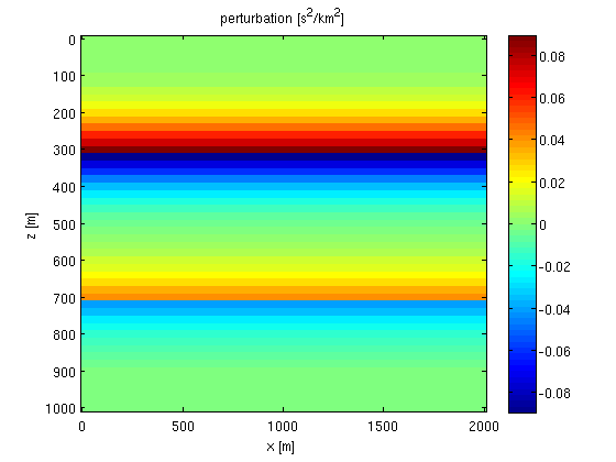
We can model linearized data by using the Jacobian. First we define a smoothed model and reflectivity.

% smoothing operator
S = opKron(opSmooth(n(2),50),opSmooth(n(1),50));

% smooth model and perturbation
m0 = S*m;
dm = m - m0;

% plot
figure;
imagesc(x,z,reshape(m0,n));colorbar;
xlabel('x [m]');ylabel('z [m]');title('Smooth model [s^2/km^2]');

figure;
imagesc(x,z,reshape(dm,n));colorbar;
xlabel('x [m]');ylabel('z [m]');title('perturbation [s^2/km^2]');

The Jacobian operator is constructed as follows:

J = oppDF(m0,Q,model,1);

Remember, J is not an explicit matrix. It is simply an object that looks like a matrix to matlab. Constructing it does not require any computation. All the computations are done when multiplying it with a vector.

The linearized data is now simply given by

dD = J*dm;

dD = reshape(dD,nrec,nsrc,nfreq);

% plot
figure;
imagesc(real(dD(:,:,3)));
xlabel('source number');ylabel('receiver number');title(['Real part of data @ ' num2str(model.freq(3)) ' Hz']);

References

[1] C-H Jo,* C. Shin,* and J.H. Suh, 1996. An optimal 9-point, finite-difference, frequency-space, 2-D scalar wave extrapolator Geophysics 61(2), 529-537.