2D constant-density acoustic frequency-domain modeling, linearized modeling and imaging: Imaging

We illustrate some basic imaging capabilities on a simple layered model.

Contents

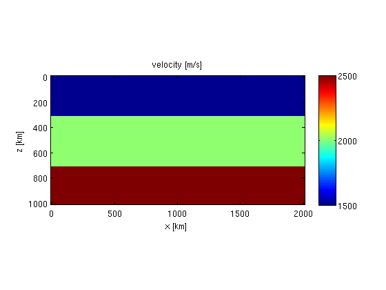
Model

We define a simple layered model:

% grid
z = 0:20:1000;
x = 0:20:2000;
[o,d,n] = grid2odn(z,x);

% velocity
v = 1500*ones(n);
v(z>300,:) = 2000;
v(z>700,:) = 2500;

% plot
figure;
imagesc(x,z,v);axis equal tight;colorbar;
xlabel('x [km]');ylabel('z [km]');title('velocity [m/s]');

Parameters for data

% gridded slowness-squared values [km^2/s^2]
m = 1e6./v(:).^2;

% model grid
model.o = o;
model.d = d;
model.n = n;

% absorbing boundary
model.nb = [20 20];

% source/receiver grid
model.zsrc = 15;
model.xsrc = 500:100:1500;
model.zrec = 5;
model.xrec = 0:15:2000;

% frequencies
model.freq = [4:2:15];

% wavelet
model.f0 = 10;
model.t0 = 0.01;

% source matrix
Q = speye(length(model.xsrc));

% make data
D = F(m,Q,model);

Reverse-time-migration

We can perform RTM by applying the adjoint of the Jacobian to the data. We model data for a smooth background model:

% smoothing operator
S = opKron(opSmooth(n(2),50),opSmooth(n(1),50));

% smooth model
m0 = S*m;

% data and Jacobian for smooth model
[D0,J0] = F(m0,Q,model);

Remember, J0 is not an explicit matrix. It is simply an object that looks like a matrix to matlab. Constructing it does not require any computation. All the computations are done when multiplying it with a vector.

Now, the RTM image is given by

dm = J0'*(D-D0);

% plot
figure;
imagesc(x,z,reshape(dm,n));axis equal tight;colormap(gray);
xlabel('x [m]');ylabel('z [m]');title('RTM image');

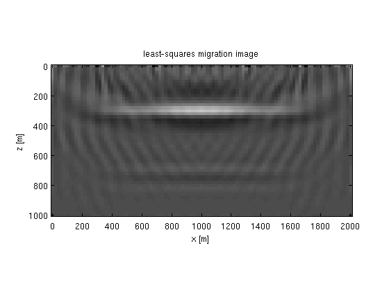
Least-squares migration

Using the Jacobian, we can perform least-squares migration with lsqr as follows

dm = lsqr(J0,D-D0,1e-6,2);

figure;
imagesc(x,z,reshape(dm,n));axis equal tight;colormap(gray);
xlabel('x [m]');ylabel('z [m]');title('least-squares migration image');

lsqr stopped at iteration 2 without converging to the desired tolerance 1e-06
because the maximum number of iterations was reached.
The iterate returned (number 2) has relative residual 0.73.