Written by Bas Peters (bpeters {at} eos.ubc.ca), February 2014.

Contents

Wavefield Reconstruction Imaging

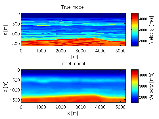
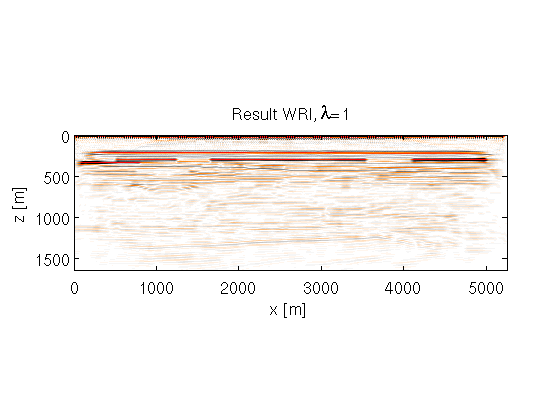
This script will show examples of migration in the BG Compass model. The theory behind this imaging method is described in [1],[2] and the example shown here was previously presented in [3]. The images are formed as follows: We use the Wavefield Reconstructing Inversion objective functional

\( \bar{\phi}_{\lambda}(\mathbf{m}) = \frac{1}{2}\| P \bar{\mathbf{u}} -\mathbf{d}\|^{2}_{2} + \frac{\lambda^2}{2}\|A(\mathbf{m})\bar{\mathbf{u}}-\mathbf{q}\|^{2}_{2} \)

of which we calculate its gradient with respect to the model parameters (slowness squared)

\( I_{\lambda}=\nabla_{\mathbf{m}} \bar{\phi}_\lambda = \lambda^2 G(\mathbf{m},\bar{\mathbf{u}})^* \big( A(\mathbf{m})\bar{\mathbf{u}} -\mathbf{q} \big) \)

This gradient is our image. The field \( \bar{\mathbf{u}} \) is defined as:

\( \bar{\mathbf{u}}= (\lambda^2 A(\mathbf{m})^* A(\mathbf{m}) + P^*P)^{-1} (\lambda^2 A(\mathbf{m})^* \mathbf{q} + P^* \mathbf{d}) \)

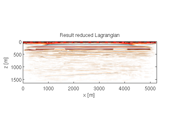
Note that a different choice of \( \lambda \) will give us a different image.The results are compared to the image obtained by Reverse-Time Migration. This method also computes the image as the gradient of an objective functional. It is the gradient of a reduced Lagrangian least-squares objective:

\( \phi_{r}(\mathbf{m})=\frac{1}{2}\| P A^{-1}\mathbf{q} - \mathbf{d}\|^{2}_{2}, \)

and the gradient can be computed using an adjoint-state method as

\( I_r = \nabla_{\mathbf{m}}\phi_r(\mathbf{m}) = G(\mathbf{m},\mathbf{u})^* \mathbf{v} \)

where \( \mathbf{v}= -A^{-*} P^*(P \mathbf{u}- \mathbf{d}) \) is the adjoint-field.

The modeling used in this example is described in https://www.slim.eos.ubc.ca/SoftwareDemos/applications/Modeling/2DAcousticFreqModeling/modeling.html.

System requirements:

close all

%plot true and background velocity
v0 = reshape(1e3./sqrt(m0),n); %convert back to velocity in [m/s]
figure(1)
subplot(2,1,1);set(gca,'Fontsize',14)
imagesc(x,z,v,[1500 4500]);colorbar;title('True model')
xlabel('x [m]');ylabel('z [m]');axis equal tight;h = colorbar;ylabel(h, 'Velocity [m/s]','FontSize',14);
subplot(2,1,2);set(gca,'Fontsize',14)
imagesc(x,z,v0,[1500 4500]);colorbar;title(['Initial model'])
xlabel('x [m]');ylabel('z [m]');axis equal tight;h = colorbar;ylabel(h, 'Velocity [m/s]','FontSize',14);

%plot migration results
np = gpen./hpen;            %Gauss-Newton image (for sufficiently small $$ \lambda$$ ).
gr = reshape((gred),n);     %Reduced Lagrangian image (RTM)
gp = reshape((gpen),n);     %WRI method image
np = reshape(np,n);
hp = reshape(hpen,n);       %WRI Gauss-Newton Hessian (diagonal)

%optional: take the vertical diff to get rid of constant trends in the
%result
gr=diff(diff(gr));
gp=diff(diff(gp));
np=diff(diff(np));

figure(2)
set(gca,'Fontsize',14)
imagesc(x,z,(gr),[-3e5 3e5]);colormap prx;title('Result reduced Lagrangian')
xlabel('x [m]');ylabel('z [m]');axis equal tight;

figure(3);set(gca,'Fontsize',14)
imagesc(x,z,(gp),[-8e0 8e0]);colormap prx;title(['Result WRI, \lambda=',num2str(params.lambda)])
xlabel('x [m]');ylabel('z [m]');axis equal tight;

figure(4);set(gca,'Fontsize',14)
imagesc(x,z,(1e5*np),[-15 15]);colormap prx;title(['Result WRI (GN), \lambda=',num2str(params.lambda)])
xlabel('x [m]');ylabel('z [m]');axis equal tight;

References

[1] Tristan van Leeuwen, Felix J. Herrmann, Geophysical Journal International,2013. Mitigating local minima in full-waveform inversion by expanding the search space.

[2] Tristan van Leeuwen, Felix J. Herrmann. 2013. A penalty method for PDE-constrained optimization.

[3] Bas Peters, Felix J. Herrmann, Tristan van Leeuwen. EAGE, 2014. Wave-equation based inversion with the penalty method: adjoint-state versus wavefield-reconstruction inversion.