Sparsity promoting LSRTM with linearized Bregman

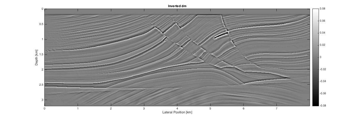
Example script for running least-squares RTM with sparsity promotion and source subsampling on the Marmousi model.

Author: Philipp Witte Date: February 2016

Contents

Set paths to result,data,model etc.

clear all; clc;
rng('default')

% Load software release functions
% SLIM_APPS.tools.algorithms.TimeModeling
addpath(genpath('~/SLIM-release-apps'));

% paths  and name of results and snapshots
snapshotX = 'UpdateTest_X.mat';
snapshotZ = 'UpdateTest_Z.mat';
result = 'Result.mat';
params = 'Parameters.mat';

% pull data and model
% if ~exist('../data/modelMarmousi.mat','file')
% 	cd ../data/; ! scons; cd ../examples/;
% end

% Marmousi slowness^2 model [s^2/km^2]
load modelMarmousi.mat

% Load 2D data cube [ns x nrec x nsrc]
% load ../data/linDataMarmousi.mat

Modeling parameters

Set up a structure that contains information about the velocity model and the source/receiver geometry of the input data.

% model parameters
model.o = [0, 0, 0];  % Origin [m]
model.n = [320, 800, 1];  % no. of grid points [z,x,y]
model.d = [10, 10, 10];   % grid spacing [m]
model.freesurface = 0;

% data parameters
model.f0   = 0.030; % peak frequency [MHz]
model.T= 4000;  % Recording length [ms]
model.NyqT=0:4:model.T; % Shot record time axis [ms]

% source/receiver position [m]
model.xsrc = 25:25:(n(2)*d(2));
model.zsrc = 10*ones(size(model.xsrc));
model.ysrc =  0*ones(size(model.xsrc));
model.xrec = 5:10:n(2)*d(2)-5;
model.zrec = 210;
model.yrec = 0;

% Code specific options
model.save = 'RAM'; % save wavefields in memory
model.type='full'; % acquisition geometry
model.space_order=4; % Order of Laplacian

% Domain decomposition
model.ddcompx = 1;
model.ddcompz = 1;
model.ddcompy = 1;

LSRTM parameters

Define the number of iterations for the linearized Bregman method, as well as the L2 norm of the noise , the thresholding value and the number of sources per iteration. Furthermore, set up a structure that defines which preconditioners are used. All preconditioners are disabled as default and can be enabled by setting them to '1'.

% LSRTM options
options.iterations = 40;
options.lambda = [];
options.sigma = 0;
options.numShots = 8;   % No. of shots per Bregman iteration
options.snapshotX = snapshotX;
options.snapshotZ = snapshotZ;

% Preconditioners
precon.modelDepth = 1;
precon.modelTopmute = 1;
precon.dataScaling = 1;
precon.dataTopmute = 1;

Setup grid and modeling options

% Calculate optimal grid size and time step
[m,model,dmTrue]=Setup_CFL(m,model,dm);

% Source wavelet
q=sp_RickerWavelet(model.f0,1/model.f0,model.dt,model.T);

CFL conditions gives dt = 0.57736ms and d = 5  5  5 m 
Velocity interpolated on new grid

Call algorithm and save results

Runtime per iteration (one demigration and one migration) for this example was ~20 minutes.

% [dm,info] = linbregLSRTM(dData,model,m0,q,precon,options);
% save(result,'dm','info');
% save(params,'model');

Plot results

load Result.mat
load Parameters.mat

x = linspace(0,7.995,model.n(2));
z = linspace(0,3.195,model.n(1));

% true image
figure('Position',[400,400,1200,400]);
imagesc(x,z,reshape(-dmTrue,model.n));
xlabel('Lateral Position [km]'); ylabel('Depth [km]');
colormap gray; caxis([-1 1]*8e-2);  colorbar
title('True dm');

% lsrtm image
figure('Position',[400,400,1200,400]);
imagesc(x,z,dm);
xlabel('Lateral Position [km]'); ylabel('Depth [km]');
colormap gray; caxis([-1 1]*8e-2);  colorbar
title('Inverted dm');

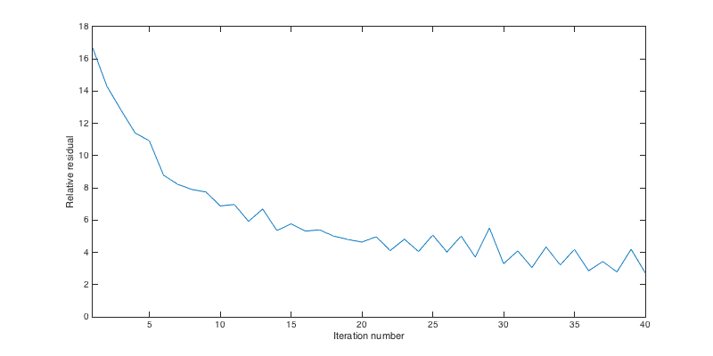
figure('Position',[400,400,800,400]);
plot(info.residual)
xlabel('Iteration number'); ylabel('Relative residual');
axis([1 40 0 18]);