Fast least-squares imaging with source estimation using multiples: examples and results

Examples included in the software.

Author: Ning Tu (tning@eos.ubc.ca) Date: Dec/17/2015

Contents

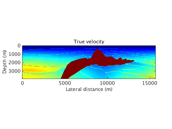
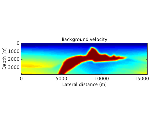
Examples using the SEG/EAGE salt model

nt = 2001;
dt = 0.004;
df = 1/(nt*dt);
freq = df:df:12;
nf = length(freq);
f0 = 5;
t0 = -0.25;
trueS = ricker_freq(f0,t0,freq);
trueS = trueS(:);

% These are the true and the background model
dz = 24.384;
dx = 24.384;
b_kz = 0.05/(2*dz);

model_file = ['../data/model.mat'];
load(model_file)
m = vel_true;
m0 = vel_bg;
m = 1e6./(m.^2);
m0 = 1e6./(m0.^2);
dm_true = m-m0;

show_model(vel_true,'jet',dz,dx)
caxis([1.5 4.5])
title('True velocity')
xlabel('Lateral distance (m)')
ylabel('Depth (m)')
set_my_figure

show_model(vel_bg,'jet',dz,dx)
caxis([1.5 4.5])
title('Background velocity')
xlabel('Lateral distance (m)')
ylabel('Depth (m)')
set_my_figure

Showing a velocity or density model...
Showing a velocity or density model...

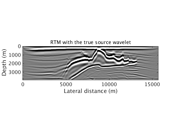
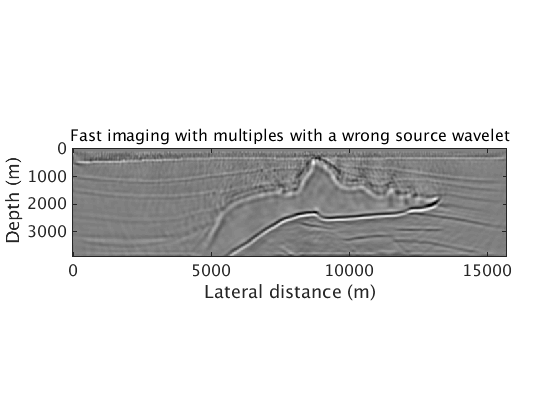
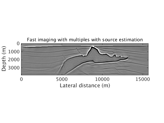
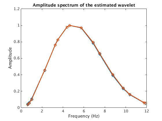
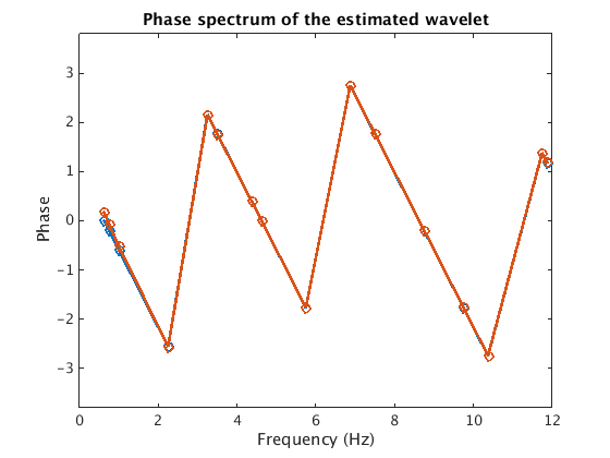
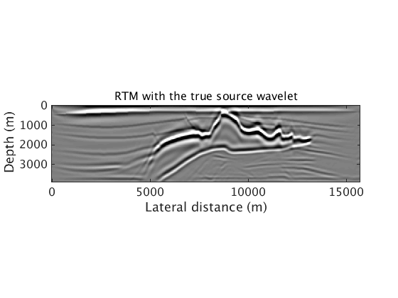
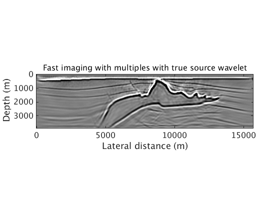
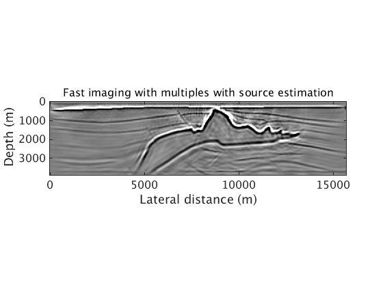
Ideal case: data synthesis and inversion using the same linearized modelling

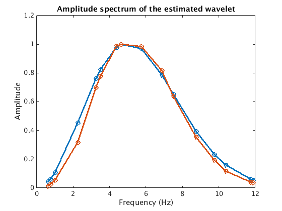
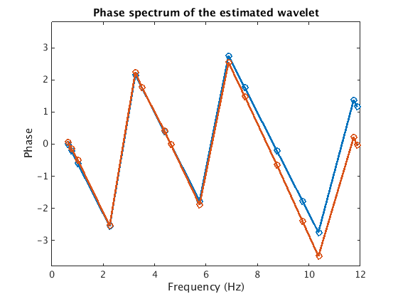
% RTM image
result = ['../results/precooked/segsalt/linear_RTM.mat'];
load(result,'dm_RTM')
dm = dm_RTM.*repmat(vec(1:size(dm_RTM,1)).^1, [1 size(dm_RTM,2)]);
dm = hp1D_z(dm,dz,dx,b_kz);
show_model(dm,'gray',dz,dx)
caxis([-1 1]*3e8)
set_my_figure
title('RTM with the true source wavelet')
xlabel('Lateral distance (m)')
ylabel('Depth (m)')

% Inversion image with the true source wavelet
result = ['../results/precooked/segsalt/linear_trueQ_GaussianEnc2_denoised.mat'];
load(result,'dm')
show_model(dm,'gray',dz,dx)
caxis([-1 1]*0.06)
set_my_figure
title('Fast imaging with multiples with true source wavelet')
xlabel('Lateral distance (m)')
ylabel('Depth (m)')

% Inversion image with a wrong source wavelet
result = ['../results/precooked/segsalt/linear_wrongQ2_GaussianEnc2_denoised.mat'];
load(result,'dm')
show_model(dm,'gray',dz,dx)
caxis([-1 1]*0.06)
set_my_figure
title('Fast imaging with multiples with a wrong source wavelet')
xlabel('Lateral distance (m)')
ylabel('Depth (m)')

% Inversion image with source estimation
result = ['../results/precooked/segsalt/linear_estQ_GaussianEnc2_denoised.mat'];
load(result,'dm')
show_model(dm,'gray',dz,dx)
caxis([-1 1]*0.3)
set_my_figure
title('Fast imaging with multiples with source estimation')
xlabel('Lateral distance (m)')
ylabel('Depth (m)')

% plot the estimated source wavelet
result_file = ['../results/precooked/segsalt/linear_estQ_GaussianEnc2.mat'];
load(result_file,'S_f_full','S_f','fidx')
figure
plot(freq(fidx),abs([trueS(fidx)/max(trueS(fidx)),S_f/max(S_f)]),'-o','linewidth',2)
xlabel('Frequency (Hz)')
ylabel('Amplitude')
axis([0 12 0 1.2])
title('Amplitude spectrum of the estimated wavelet')
figure
plot(freq(fidx),angle([trueS(fidx)/max(trueS(fidx)),S_f/max(S_f)]),'-o','linewidth',2)
xlabel('Frequency (Hz)')
ylabel('Phase')
axis([0 12 -3.8 3.8])
title('Phase spectrum of the estimated wavelet')

Showing a velocity or density model...
Showing a velocity or density model...
Showing a velocity or density model...
Showing a velocity or density model...

More realistic case: data sythesis using iWave, inversion using SLIM modelling

% RTM image
result = ['../results/precooked/segsalt/iwave_RTM.mat'];
load(result,'dm_RTM')
dm = -dm_RTM.*repmat(vec(1:size(dm_RTM,1)).^1, [1 size(dm_RTM,2)]);
dm = hp1D_z(dm,dz,dx,b_kz);
show_model(dm,'gray',dz,dx)
caxis([-1 1]*2e10)
set_my_figure
title('RTM with the true source wavelet')
xlabel('Lateral distance (m)')
ylabel('Depth (m)')

% Inversion image with the true source wavelet
result = ['../results/precooked/segsalt/iwave_finv_trueQ_GaussianEnc2_denoised.mat'];
load(result,'dm')
show_model(-dm,'gray',dz,dx)
caxis([-1 1]*1.2)
set_my_figure
title('Fast imaging with multiples with true source wavelet')
xlabel('Lateral distance (m)')
ylabel('Depth (m)')

% Inversion image with source estimation
result = ['../results/precooked/segsalt/iwave_finv_estQ_GaussianEnc2_denoised.mat'];
load(result,'dm')
show_model(-dm,'gray',dz,dx)
caxis([-1 1]*15)
set_my_figure
title('Fast imaging with multiples with source estimation')
xlabel('Lateral distance (m)')
ylabel('Depth (m)')

% plot the estimated source wavelet
result_file = ['../results/precooked/segsalt/iwave_finv_estQ_GaussianEnc2.mat'];
load(result_file,'S_f_full','S_f','fidx')
figure
plot(freq(fidx),abs([trueS(fidx)/max(trueS(fidx)),S_f/max(S_f)]),'-o','linewidth',2)
xlabel('Frequency (Hz)')
ylabel('Amplitude')
axis([0 12 0 1.2])
title('Amplitude spectrum of the estimated wavelet')
figure
ang1 = angle(trueS(fidx)/max(trueS(fidx)));
ang2 = angle(S_f/max(S_f));
ang2(14)=ang2(14)-2*pi;
plot(freq(fidx),[ang1, ang2],'-o','linewidth',2)
xlabel('Frequency (Hz)')
ylabel('Phase')
axis([0 12 -3.8 3.8])
title('Phase spectrum of the estimated wavelet')

Showing a velocity or density model...
Showing a velocity or density model...
Showing a velocity or density model...

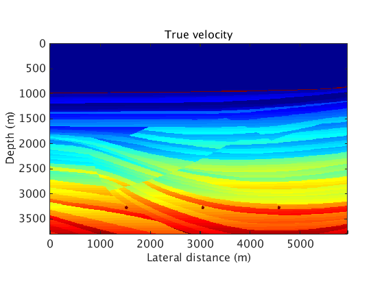
Examples using the Sigsbee 2B model

nt = 1024;
dt = 0.008;
df = 1/(nt*dt);
freq = df:df:38;
nf = length(freq);
f0 = 15;
t0 = 0;
trueS = ricker_freq(f0,t0,freq);
trueS = trueS(:);

% These are the true and the background model
dz = 7.62;
dx = 7.62;

model_file = ['../data/sigsbee_nosalt_model.mat'];
load(model_file)
m = vel_true;
m0 = vel_bg;
m = 1e6./(m.^2);
m0 = 1e6./(m0.^2);
dm_true = m-m0;

show_model(vel_true,'jet',dz,dx)
caxis([1500 2500])
title('True velocity')
xlabel('Lateral distance (m)')
ylabel('Depth (m)')
set_my_figure

show_model(vel_bg,'jet',dz,dx)
caxis([1500 2500])
title('Background velocity')
xlabel('Lateral distance (m)')
ylabel('Depth (m)')
set_my_figure

Showing a velocity or density model...
Showing a velocity or density model...

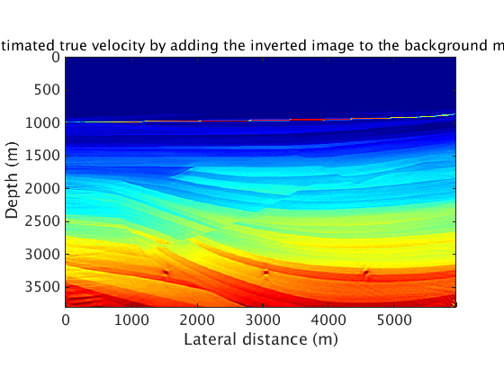
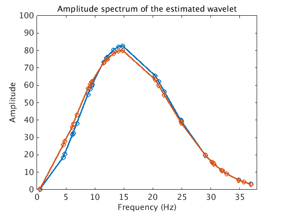
Ideal case: synthesis and inversion with the same linearized modelling engine

% image
result = ['../results/precooked/sigsbee/MigTotalLinear_26ss31freq_EstQ_GausEnc_denoised.mat'];
load(result,'dm')
show_model(dm,'gray',dz,dx)
caxis([-1 1]*0.06)
set_my_figure
title('Fast imaging with multiples with source estimation')
xlabel('Lateral distance (m)')
ylabel('Depth (m)')

% estimate of the true velocity model
vel_true_est = sqrt(1e6./(1e6./vel_bg.^2+dm));
show_model(vel_true_est,'jet',dz,dx)
caxis([1500 2500])
set_my_figure
title('Estimated true velocity by adding the inverted image to the background model')
xlabel('Lateral distance (m)')
ylabel('Depth (m)')

% estimated source wavelet

result = ['../results/precooked/sigsbee/MigTotalLinear_26ss31freq_EstQ_GausEnc.mat'];
load(result,'S_f_full','S_f','fidx')
figure
plot(freq(fidx),abs([trueS(fidx),S_f]),'-o','linewidth',2)
xlabel('Frequency (Hz)')
ylabel('Amplitude')
axis([0 38 0 100])
title('Amplitude spectrum of the estimated wavelet')
set_my_figure
figure
plot(freq(fidx),angle([trueS(fidx),S_f]),'-o','linewidth',2)
xlabel('Frequency (Hz)')
ylabel('Phase')
axis([0 38 -3.8 3.8])
title('Phase spectrum of the estimated wavelet')
set_my_figure

Showing a velocity or density model...
Showing a velocity or density model...

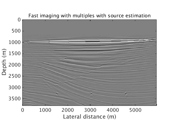
More realistic case: data synthesized using iWave, inverted using SLIM modelling engine

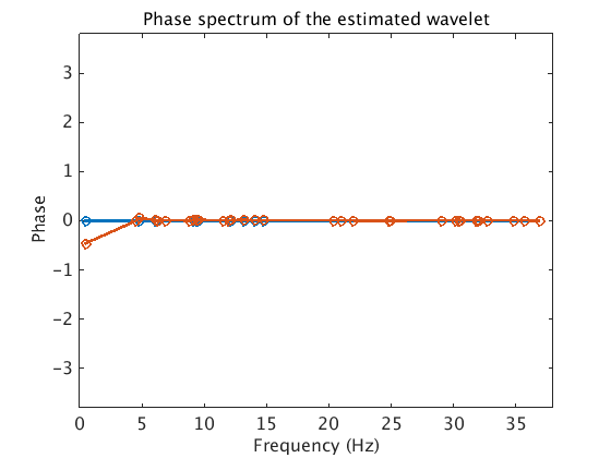
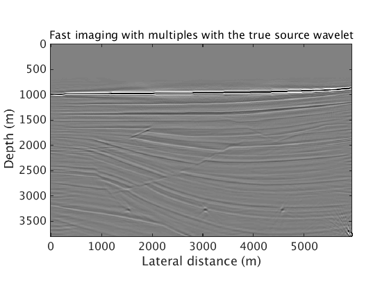
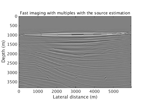
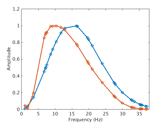
% with true source
result = ['../results/precooked/sigsbee/MigTotalFD_iwave_26ss31freq_bg_TrueQ_GaussianEnc_denoised.mat'];
load(result,'dm')
show_model(dm,'gray',dz,dx)
caxis([-1 1]*0.06)
set_my_figure
title('Fast imaging with multiples with the true source wavelet')
xlabel('Lateral distance (m)')
ylabel('Depth (m)')

% with source estimation
result = ['../results/precooked/sigsbee/MigTotalLinear_26ss31freq_EstQ_GausEnc_denoised.mat'];
load(result,'dm')
show_model(dm,'gray',dz,dx)
caxis([-1 1]*0.06)
set_my_figure
title('Fast imaging with multiples with the source estimation')
xlabel('Lateral distance (m)')
ylabel('Depth (m)')

% estimated source wavelet
result = ['../results/precooked/sigsbee/MigTotalFD_iwave_26ss31freq_EstQ_GausEnc_wAmpCor.mat'];
load(result,'S_f_full','S_f','fidx')
figure
plot(freq(fidx),abs([trueS(fidx)/max(trueS(fidx)),S_f/max(S_f)]),'-o','linewidth',2)
xlabel('Frequency (Hz)')
ylabel('Amplitude')
axis([0 38 0 1.2])
title('')
set_my_figure
figure
angSf = angle(S_f);
plot(freq(fidx),[angle(trueS(fidx)),angSf],'-o','linewidth',2)
xlabel('Frequency (Hz)')
ylabel('Phase')
axis([0 38 -3.8 3.8])
title('')
set_my_figure

Showing a velocity or density model...
Showing a velocity or density model...

Sensitivity to initial guess of the source wavelet

% two wrong intial guesses of the source wavelet
nt = 10231;
dt = 0.0008;
df = 1/(nt*dt);
freq = df:df:38;
nf = length(freq);
freq_full = 0:df:df*floor(nt/2);
freq_mask = get_subset_mask(freq_full,freq);
opFT1D = opFFTsym_conv_mask(nt,freq_mask);

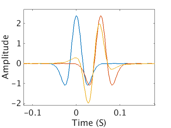
true wavelet and initial guesses

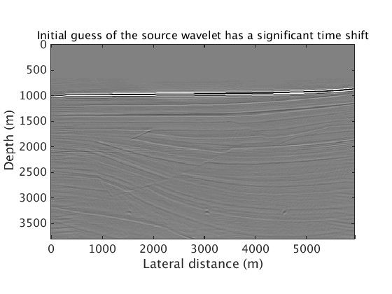
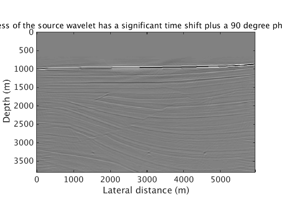
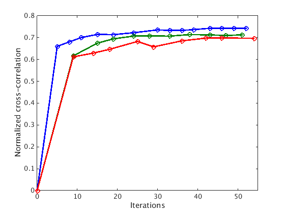
f0 = 15;
t0 = 0;
trues = ricker_freq(f0,t0,freq);
trues = fftshift(opFT1D'*trues(:));
f1 = 15;
t1 = -0.056;
ig1 = ricker_freq(f1,t1,freq);
ig1 = fftshift(opFT1D'*ig1(:));
f2 = 15;
t2 = -0.04;
ig2 = ricker_freq(f2,t2,freq);
ig2 = opFT1D'*ig2(:);
ig2 = hilbert(ig2);
ig2 = fftshift(imag(ig2));
t_axis = fftshift(0:dt:dt*(nt-1));
t_axis(t_axis>dt*nt/2) = t_axis(t_axis>dt*nt/2) - dt*nt;
figure
plot(t_axis,[trues,ig1,ig2],'linewidth',2)
axis([-0.12 0.18 -2.1 2.7])
set_my_figure(gca,20)
xlabel('Time (S)')
ylabel('Amplitude')

% Initial guess of the source wavelet has a significant time shift
result = ['../results/precooked/sigsbee/MigTotalFD_iwave_26ss31freq_EstQ_GausEnc_wAmpCor_IG1_BS_denoised.mat'];
load(result,'dm')
show_model(dm,'gray',dz,dx)
caxis([-1 1]*0.06)
title('Initial guess of the source wavelet has a significant time shift')
xlabel('Lateral distance (m)')
ylabel('Depth (m)')

% Initial guess of the source wavelet has a significant time shift plus a 90 degree phase rotation
result = ['../results/precooked/sigsbee/MigTotalFD_iwave_26ss31freq_EstQ_GausEnc_wAmpCor_IG2_BS_denoised.mat'];
load(result,'dm')
show_model(dm,'gray',dz,dx)
caxis([-1 1]*0.06)
title('Initial guess of the source wavelet has a significant time shift plus a 90 degree phase rotation')
xlabel('Lateral distance (m)')
ylabel('Depth (m)')

% Normalized cross-correlation along inversion
% true pert
load(model_file)
truepert = 1e6./vel_true.^2-1e6./vel_bg.^2;
truepert = [repmat(truepert(1,:),[3 1]);truepert];
truepert = truepert(:);

% trueQ
result_file = ['../results/precooked/sigsbee/MigTotalFD_iwave_26ss31freq_bg_TrueQ_GaussianEnc.mat'];
load(result_file,'info')
result_file = ['../results/precooked/sigsbee/MigTotalFD_iwave_26ss31freq_bg_TrueQ_GaussianEnc_snapshots.mat'];
load(result_file,'saved')
nupdates = size(saved,2);

corvec_trueQ = zeros(nupdates,1);
angvec_trueQ = zeros(nupdates,1);
for i = 2:nupdates
    [corvec_trueQ(i) angvec_trueQ(i)] = myncc(truepert,saved(:,i));
end
iteraxis_trueQ = zeros(nupdates,1);
iteraxis_trueQ(2:end) = cumsum(info.innerloop_list);

% IG1
result_file = ['../results/precooked/sigsbee/MigTotalFD_iwave_26ss31freq_EstQ_GausEnc_wAmpCor_IG1_BS.mat'];
load(result_file,'info')
result_file = ['../results/precooked/sigsbee/MigTotalFD_iwave_26ss31freq_EstQ_GausEnc_wAmpCor_IG1_BS_snapshots.mat'];
load(result_file,'saved')
nupdates = size(saved,2);

corvec_ig1 = zeros(nupdates,1);
angvec_ig1 = zeros(nupdates,1);
for i = 2:nupdates
    [corvec_ig1(i) angvec_ig1(i)] = myncc(truepert,saved(:,i));
end
iteraxis_ig1 = zeros(nupdates,1);
iteraxis_ig1(2:end) = cumsum(info.innerloop_list);

% IG2
result_file = ['../results/precooked/sigsbee/MigTotalFD_iwave_26ss31freq_EstQ_GausEnc_wAmpCor_IG2_BS.mat'];
load(result_file,'info')
result_file = ['../results/precooked/sigsbee/MigTotalFD_iwave_26ss31freq_EstQ_GausEnc_wAmpCor_IG2_BS_snapshots.mat'];
load(result_file,'saved')
nupdates = size(saved,2);

corvec_ig2 = zeros(nupdates,1);
angvec_ig2 = zeros(nupdates,1);
for i = 2:nupdates
    [corvec_ig2(i) angvec_ig2(i)] = myncc(truepert,saved(:,i));
end
iteraxis_ig2 = zeros(nupdates,1);
iteraxis_ig2(2:end) = cumsum(info.innerloop_list);

figure
plot(iteraxis_trueQ,corvec_trueQ,'-ob','linewidth',2)
hold on
plot(iteraxis_ig1,corvec_ig1,'-o','color',[0 0.5 0],'linewidth',2)
plot(iteraxis_ig2,corvec_ig2,'-o','color',[1 0 0],'linewidth',2)
axis([0 55 0 0.8])
xlabel('Iterations')
ylabel('Normalized cross-correlation')

Showing a velocity or density model...
Showing a velocity or density model...